Segment analysis in experimentation: how to avoid fooling yourself

Dimension splits can surface what your Average Treatment Effect hides, or fool you with noise. How to avoid cherry-picking your results, correct for multiple tests, and steer clear of bad controls.

Why your experiment results look different across segments

Your experiment's Average Treatment Effect (ATE) is just that, an average. As we wrote in the previous piece, behind a flat or modest headline result, users can be having very different experiences. Real gains for some, real losses for others, with the effects canceling out in aggregate. How do you actually find those differences, and how do you know when you've found something real?

The answer, in most experiments, is dimension splits: cutting your results by user properties like market, device, plan tier, or account age. It's a natural instinct and a reasonable one. The problem is that the same dataset that contains real signals also contains noise, and noise has a habit of looking like signal when you cut the data enough ways.

That doesn't mean you shouldn't do it. There are three good reasons to look at segment-level effects:

1. Understanding the mechanism. Why did this feature work, and for whom?
2. Informing a rollout decision. Should this go to everyone, or only to certain users?
3. Assessing commercial value when short-term metrics fall short. Some features matter most to your most valuable users, and a single headline number won't show you that.

To make these questions concrete, we'll use a running example throughout: an upsell banner prompting users to join a paid loyalty program.

Whatever your reason for splitting, what you're estimating in each segment is its own Conditional Average Treatment Effect (CATE): the treatment effect for users in that subgroup rather than for the full population. And one caveat applies no matter how you slice: segment samples are smaller than the full experiment population, so estimates are noisier and you have less power to detect an effect of a given size.

This piece covers three ways those splits can mislead you. Each calls for a different response.

Before the experiment: pre-specify your segments

The most defensible approach to segment analysis starts before the experiment runs. You identify the dimensions you want to examine and write down the hypothesis behind each. For the loyalty program upsell banner example, at least two dimensions make sense: recent buyers (those who made at least one purchase in the 30 days before launch), who may respond more strongly because they are already more loyal; and market, because the loyalty program is more developed in some countries. We pre-specify these dimensions because we have clear hypotheses.

Why write the hypothesis down?

Pre-specifying protects against a specific failure mode: cherry-picking. When you choose which dimensions to examine after seeing the results, it's easy, even unintentionally, to frame a fishing expedition as a deliberate analysis. You report back the dimensions with interesting results, but quietly discard the ones without. Writing down your dimensions and hypotheses before the experiment starts makes that impossible: everyone can see you made the choice before the results could influence you. 

Pre-specifying doesn't solve everything, though. Pre-specify 20 markets and you'd expect roughly one to come up significantly by chance, even if the feature does nothing anywhere. That's the multiple testing problem, and pre-specifying only means you're facing it honestly.

Which correction fits the decision?

When the goal is a per-segment rollout decision rather than understanding the mechanism, the stakes change. You're making an independent call for each segment: does this market get the feature, or not? A wrong call ships a feature to users it doesn't help.

The obvious fix is to raise the bar. Instead of calling a result significant at 5%, demand 1%. That instinct is right, and it's essentially what a multiple testing correction does. The difference is that a correction sets the bar for you, based on how many segments you tested and which kind of mistake you're trying to avoid. Set it by hand and you're guessing. Too loose and you roll out to segments that were noise. Too strict and you miss the segments where it worked, which is a real risk when each segment is a fraction of your sample.

So the question isn't whether to correct, it's which correction matches the decision you're making. The table below summarizes the two standard approaches. Both are frequentist, framed around p-values. GrowthBook's Bayesian engine has a direct counterpart for each, which we note as we go.

For per-segment rollout decisions, FDR is probably more natural. When you're making independent calls for potentially many segments, a small proportion of incorrect rollouts is an acceptable cost as long as most are right. The principle generalizes: match the correction to the decision rather than applying one uniformly.

The Bayesian equivalent

The same decision carries over to GrowthBook's Bayesian engine without any p-values. Each segment reports a Chance to Win, the posterior probability that the variation beats control. The posterior probability that a given rollout is a mistake is therefore 1 − Chance to Win. Rank the segments by Chance to Win and roll out down the list until the running average of (1 − Chance to Win) reaches the false discovery rate you're willing to accept. That average is the expected share of your rollouts that aren't real. It is the same notion of error Benjamini-Hochberg targets, read off the posterior instead of from p-values.

One assumption underpins that number. If your prior is flat, you are treating every effect size as equally plausible before you look. Scan twenty segments on that assumption and the top of your list will look better than it deserves to. A prior centered at no effect corrects some of this, because it pulls the noisiest segments toward zero hardest. Exactly how hard to pull is an open debate.

In practice, very few experimentation platforms apply any correction to dimension splits at all; most treat them as exploratory by default. GrowthBook applies correction within each dimension breakdown when the metric is a primary metric. However, it corrects within each dimension separately, not across all dimensions at once. For FWER users that's something to bear in mind: each additional dimension you run adds more chances for a false positive to slip through. For FDR the concern is much more limited, since you're controlling a proportion rather than a count.

After the experiment: how should you explore post-hoc?

Once an experiment finishes and you see the main results, you instinctively want to start slicing. Maybe the overall effect was smaller than expected, or it moved in an unexpected direction, or you're just trying to understand who moved the number. That's a useful impulse. This section isn't an argument against exploratory analysis, it's about how to do it without fooling yourself.

Exploratory analysis is harder to keep honest, because the protection you had before is gone. Pre-specifying made cherry-picking impossible to hide. Post-hoc, you're slicing after the fact, which is, in all but name, a fishing expedition. Even though it might not feel like one. The multiple testing problem hasn't gone anywhere either, and now nobody's counting. With pre-specified markets you knew how many tests you were running. Post-hoc slicing is open-ended: you cut by device, then tenure, then market, and by the time you cut by purchase frequency you have forgotten about device.

How do you explore honestly?

What changes is the goal. You're generating hypotheses now, not confirming them, so the question is no longer whether a segment cleared a significance threshold, and formal corrections aren't the tool for that job. Read the unadjusted intervals directly: the point estimate is the candidate signal, its width is the noise around it, and you judge each segment by how far it stands out. In GrowthBook's Bayesian engine, rank by Chance to Win and read the list the same way. Then say it out loud, to yourself and your audience, that you're ranking candidates rather than confirming findings. Keep one caveat in mind: the more segments you scan, the more spurious front-runners appear at the top of the list. Thus, a strong result is a reason to run a confirmatory test, not a finding in itself.

Report every cut you ran

Be transparent about what you actually ran. Report how many cuts you made. "We sliced by five dimensions post-hoc and the recent buyer segment showed the strongest signal" gives anyone reading the analysis the context to calibrate. Omitting that information, even unintentionally, is how people mistake exploratory findings for confirmatory ones. A shared results interface helps, since what you ran is logged and visible to the whole team rather than only to whoever ran the analysis.

One thing should raise your confidence: convergence. When independent dimensions point to the same story, that should move you more than any correction can. Just watch for the temptation to grasp for whatever story fits the results in front of you.

Treat every post-hoc result as a hypothesis, not a finding.

Replicate. That's the bottom line for exploratory segment analysis. Design a follow-up experiment that tests the result properly: pre-specified, sized for that segment, with the appropriate correction if a rollout decision is on the table. If you're not willing to run the follow-up, you're not ready to act on the finding. A result that survives replication is something you can stand behind. What doesn't replicate remains a hypothesis.

Any segment: avoid bad controls

There's one mistake that ruins a segment analysis no matter how careful you were everywhere else: splitting on a variable that the treatment itself changed. It has nothing to do with how many tests you ran or whether you pre-specified them. If the treatment moves the dimension you're splitting on, the comparison is worthless before you start.

The loyalty program example makes this concrete. After the experiment ends, you want to know whether Top Customers responded differently to the upsell banner. Makes sense: these are the users whose behavior matters most commercially. So you define "Top Customers" as anyone who spent more than $200 over the 60 days before the analysis date. Well intended, but that window overlaps the experiment period. Some treatment-group users saw the banner, joined the loyalty program, and then bought more than they otherwise would have. The program's perks gave them a new reason to spend. Some of those users crossed the $200 threshold because of the program, not because of any prior purchasing pattern.

In the control group, Top Customers are established high spenders. In the treatment group, Top Customers now also include people the program pushed over the line during the experiment. So within the same segment label, you're comparing established high spenders against a mixed group that includes newly converted ones. Any CATE estimate for Top Customers from this comparison is biased: the two groups share a label but have different baseline intentions.

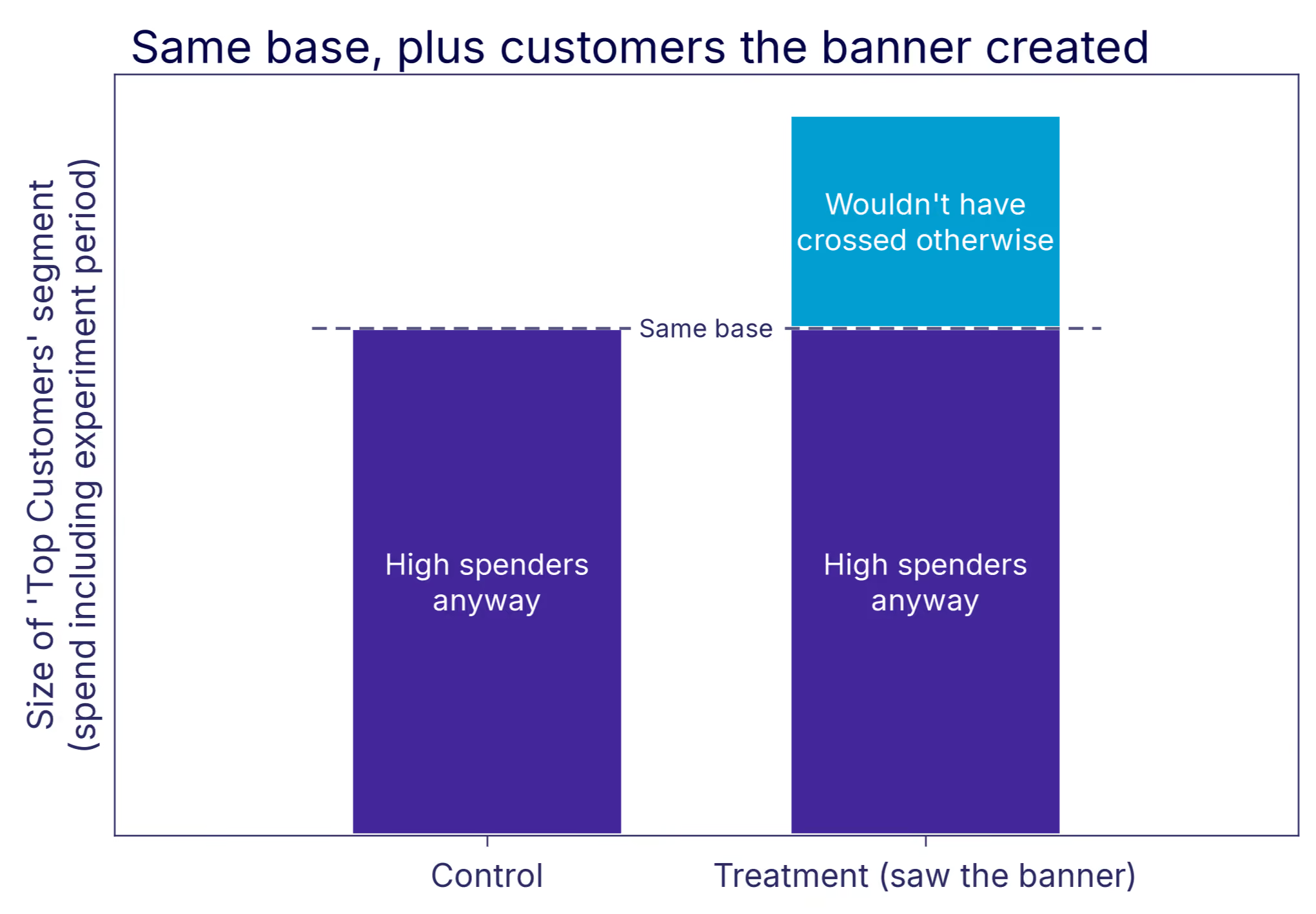
The fix is simple: segment only by pre-treatment variables. Any dimension that could plausibly have shifted in response to the treatment is off-limits, regardless of how natural it feels to look at. Top Customer status defined using spend from before the experiment started is fine. Defined using a window that overlaps the experiment period is not. With dimensions that change over time, this happens by accident. A join that picks up a user's current attribute value instead of the value at assignment time quietly reintroduces the problem.

Why post-treatment splits backfire covers the full mechanics, with a simulated experiment where every segment comes back understated.

What good segment analysis looks like

Pre-specify when you can, and apply the right correction for what you're deciding. When you explore post-hoc, do it honestly: report what you ran, treat results as hypotheses, and replicate before acting. That covers the first two reasons for running dimension splits. The third is simpler.

Think back to the Top Customers segment, defined cleanly on spend from before launch. Those users' long-run value far exceeds what a normal experiment duration can show. A feature that concentrates its effect on them can be worth shipping even when the headline ATE looks modest. That's the third reason to split: not to act on each segment, but to see whether the case for shipping to everyone is stronger than the headline number suggests.

Post-hoc slicing is exactly the kind of analysis statisticians warn you against, and the concerns above are precisely why. But the cost of never looking is just as real. Some of the most important segment effects are ones nobody had a hypothesis for, and exploration is the only way to find them. There is a more systematic way to do this. Methods like causal forests search across many dimensions at once, looking for heterogeneous treatment effects without asking you to pre-specify where to look, which takes much of the cherry-picking problem off the table. That's a topic for its own piece.

One thing worth doing this week. Pick three experiments you've already called, ideally ones where the headline came out flat or ambiguous, and open them up in exploratory mode. Not to relitigate the decision, but to build a list of segment hypotheses worth following up on. Past experiments are the cheapest source of hypotheses you have.

As Hattori Hanzō would say: any fool can pick up a blade. Knowing where to cut is the craft.