Why summing your experiment wins overstates impact

‍Sum your significant experiment wins, and you almost certainly overstate the true impact. The reason is the winner's curse: you're adding estimates that were selected for looking good. Corrections help a little, but a holdout is the real fix.

You ran forty experiments this quarter. A dozen of them had significant results, so you rolled them out. You summed up the effects, and the slide going to the leadership team says your team drove a 10% gain. Everyone celebrates. The only problem is that the number overstates the true impact.

Sure, every one of those experiments was run cleanly and read correctly. And they did pass the significance threshold. The significance threshold is what's causing the bias. The estimates you're summing are already skewed upward because lucky draws are more likely to pass than unlucky ones. So the total comes out larger than the value you actually generated.

How big of a problem can it be? Airbnb measured it: a set of winning experiments summed to 7.2%. Their de-biasing formula pulled that back to 5.3%, and a holdout put the real number near 4%. Nearly half the reported impact wasn't there, and the holdout caught more of it than the formula did.

A holdout is a simple idea: hold back a small group of users from all your new changes and measure the gap directly. There are different ways of configuring a holdout, but any of them is better than trying to infer the total impact from individual estimates.

The leadership slide is only one purpose you might have. Any time you sum individual significant results up into a single number, the same bias applies. A meta-analysis of a program, the quarter's total impact, and one team's contribution next to another's. Aggregating results that way is still useful and worth doing. This post is about doing it without overstating what you actually found. We walk through the exact mechanics of the selection-on-significance bias to give you a solid understanding. That is how you can judge, for your setting and purpose, just how big a problem you might have. And what you should do about it.

What is the winner's curse?

Every experiment hands you a measured effect, and that number is the true effect plus some noise. Run the same test next week, and you'd get a slightly different figure.

The problem arises when you look only at the significant, or shipped, results. Counterintuitive, I know. If you summed all forty estimates, winners and losers, you'd be fine. The lucky-high and the unlucky-low roughly cancel, and the total should come close to the truth. The bias enters only when selecting on statistical significance.

It is because the significance threshold isn't a random gate. An experiment is more likely to pass when the noise component pushes its estimate up than when it pulls it down. So the winners you keep aren't a fair sample of the effects you tested. On the contrary, they over-represent the ones that got a lucky draw. Gelman calls this the statistical significance filter, and the amount by which it inflates the survivors is his Type M (magnitude) error.¹

To fully understand, let's walk through the mechanics of hypothesis testing visually. Figure 1 shows the distribution of estimates you would draw from under the null, and the distribution you would draw from at a given true effect size. The scale of the x-axis is in standard errors to make it more general.

The null distribution sets the significance threshold by the chosen false positive rate (that's your α).² We can use it to visualize what part of the true-effect distribution would fall below. That's the hatched grey chunk, and these features don't get shipped. Those are your unlucky false negatives, which are more likely if your power is low (imagine the distributions widening).

The blue area illustrates the results of the significance filter. It shows the estimates that pass the significance threshold, with some luck, and get shipped. And the difference in luck is the problem. You cut away the low draws and keep the high ones, even though they have the same underlying true effect. Therefore, the average of what's shipped jumps to the right, while the center is the true effect. The average of what you shipped is higher, and it goes that way, whatever the true effect is.

This figure is constructed to show the case with 80% power, and it leads to an overestimate of 13%. The next part shows how it gets even worse with lower power.

Figure 2 shows the relationship between power and overestimated winners. At 80% power, where you'd like to be, the overstatement is the 13% we just saw. It's real, but maybe you can live with it. If the true effect comes in smaller than expected, however, the same metric and sample size give you less power. At 40% power, the survivors overstate by more than half. The reason is mechanical. A smaller true effect makes the distributions overlap more. The same thing happens if your metric is noisier than expected, or your sample is smaller than planned. Kohavi and colleagues recently replicated four widely cited 'win' patterns across eight large experiments, and the published effects came back far smaller than first reported.³

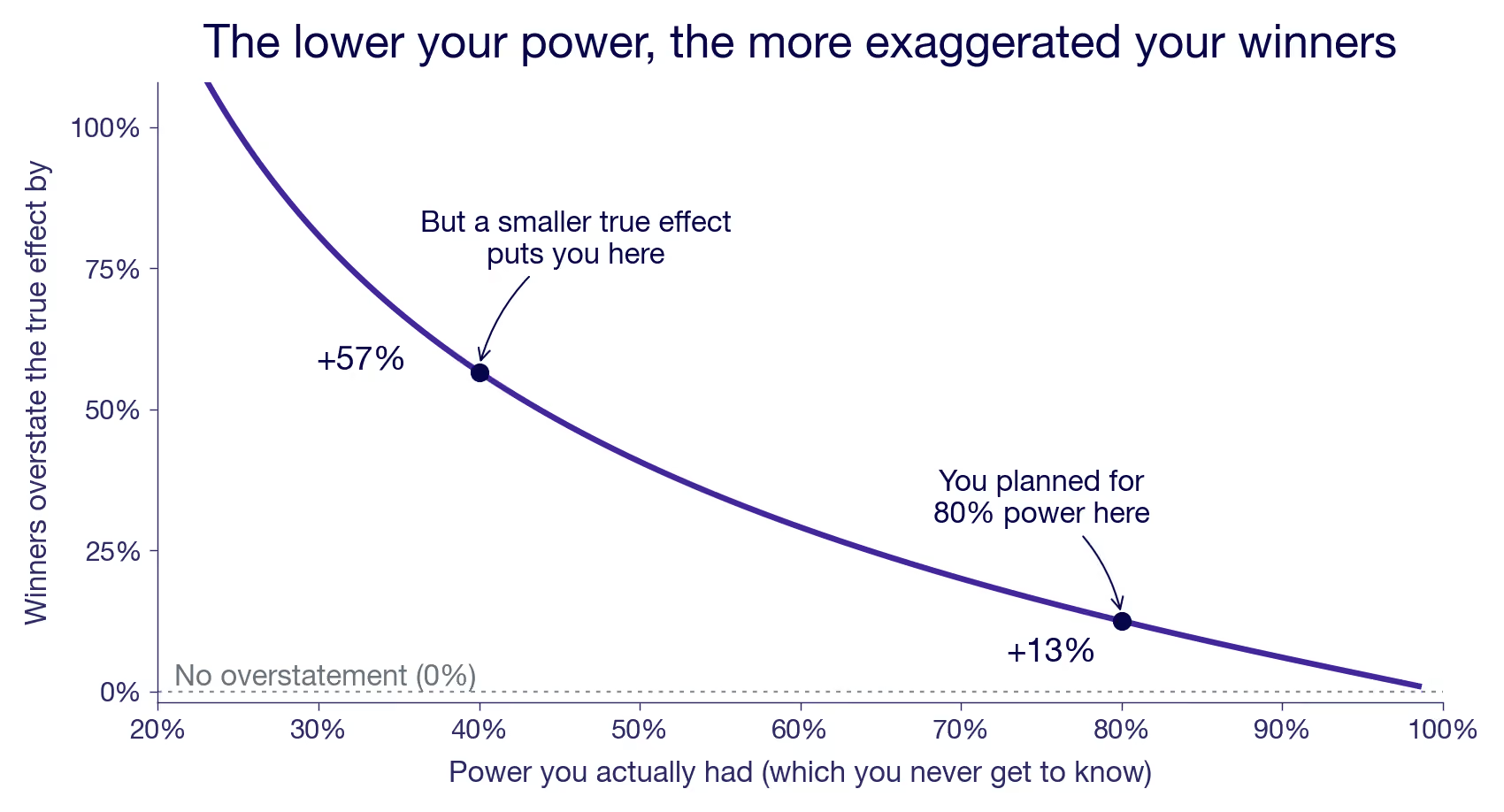
80% power is the good case, but even there, the bias is 13%. And in reality, you're probably running lower power than that on most of your experiments without knowing it. Actual power depends on the true effect you never see. Imagine the true effect actually being 40% lower than your powered MDE. Then, your realized power is 40%. Even a miss of 20% in true effect size drops your power to 60%, where you overstate your true effect by 30% when selecting on significance.

Unfortunately, you can't read the bias off a single result. A win that barely cleared could be a lucky draw from a small effect or an unlucky draw from a large one, and the number itself can't tell you which. What you can judge are the conditions you run under. If your metrics are noisy, your samples are thin, and your experiments often end inconclusive, power is scarce across the board. Your significant wins then mostly sit on the steep part of the curve. If you are generally well powered, the bias is milder. Understanding your general power situation can give you a hunch, but not the exact bias.

How to correct for the winner's curse

Can't you just correct for it? Partly. The crude way is a flat discount: Ronny Kohavi's rule of thumb is to knock at least 20% off your reported wins, the figure they used at Bing. The more careful way is to let a model do it per estimate. Switch on a proper prior in GrowthBook's Bayesian engine, and the number you read becomes the posterior mean. The raw estimate is pulled toward zero, hardest when the estimate is noisy. It shrinks on precision, not luck, which lands right on average because the noisy wins are the ones most likely inflated.

Both are more sound than estimating power from the effect you just measured and then deflating with that. Because that estimate is already inflated, it makes your power look better than it was, so the correction comes out too small. And it misses by the most, exactly when power is low. Post-hoc power like that is a known trap, not a fix.³ It's also a closed loop. The only input is the number you're trying to correct, so no new information ever enters.

What every correction shares is that it re-reads the same selected sample. To undo the selection you need a measurement that wasn't selected on. A fresh draw.

The textbook way to get one is replication. Re-run a winner and read it once, without filtering on significance, and the lucky draw that pushed it over the line the first time has no reason to repeat. That removes the bias, one experiment at a time. But replicating every winner is expensive. You would spend next quarter re-proving last quarter's, and you would still read each feature alone, with no view of what they add up to. If the purpose is to get the aggregate effect, you might as well replicate them all together in one go.

Replicating them all together is the holdout. Hold back one group from all your new changes and measure the gap once against the rollout. You give up knowing which individual winner was exaggerated, but you get the thing you were aggregating for: one honest number for the whole batch. Whether that's the total on the leadership's slide, a meta-analysis of the program, or one team's output against another's, the holdout is the complete solution for ambitious experimentation teams.

It also solves other problems for you. Some of those wins were driven by novelty effects that fade out over time. Depending on how you configure your holdout, you can solve this problem at the same time. In other experiments, your outcome metric was a proxy because your key metric was too noisy for the effect size you expected. Literally, the low power problem we have iterated here. Pooled in the holdout, these experiments either finally show an effect on the key metric, or you find out that the proxy approach doesn't work.

Because the holdout is solving multiple problems at once, there are different ways to configure it. The differences may seem subtle, and how they matter isn't obvious. That is why we cover those carefully in a separate post: what each holdout configuration actually measures.

You may have heard another reason to hold out: interactions between experiments. Several platforms list this as a key motivation. But it probably isn't moving your sum much against the holdout. When two winners interact, the sum already captures it, the same way the holdout does. That holds as long as they ran concurrently, or you shipped one before testing the next. What's left is a winner interacting with a loser, and that only biases the winner if the loser was still live during the winner's test. Because losers get switched off when they lose, often early, they should interfere less. Winners get shipped and stay on, which is the harmless case the sum handles. Interactions are worth understanding properly, and that's why we will cover them in a separate post.

Should you trust the sum of your wins?

The sum overstates what you generated, and the winner's curse is the main reason. Every winner you kept leans high because you selected it for looking good. Discounting the total or shrinking each estimate toward a prior helps, but those corrections don't solve the underlying problem. The holdout does.

Add up your wins if you like. Just think twice before you put the total on a slide.

¹ The Type M (magnitude) error, or exaggeration ratio, and the design-analysis framing the figures use are from Gelman, A., & Carlin, J. (2014). "Beyond Power Calculations: Assessing Type S (Sign) and Type M (Magnitude) Errors." Perspectives on Psychological Science, 9(6), 641–651. PDF.

² The diagram uses a two-sided 5% test, and counts only the positive, significant part as shipped, which is what you'd actually roll out. A true-zero feature lands there 2.5% of the time, not 5%. Going one-sided wouldn't change the story. It only slides the threshold to the left, to about 1.64 standard errors. That raises power and trims each winner's overstatement a little. But it buys that by doubling the rate at which pure noise ships, and the selection is still there. Drop the threshold and more marginal winners crowd into the sum, not fewer.

³ Kohavi, R., Linowski, J., Vermeer, L., Andreev, A., Dodin, M., & Furuseth, J. "Trustworthy A/B Patterns and the Winner's Curse: Lessons from Eight Large-Scale Replications." KDD 2026 (forthcoming). Preprint; doi:10.1145/3770855.3818498. Across eight high-powered replications, only two effects were significant in the expected direction and one was significant in the opposite direction. The paper quotes the same exaggeration-by-power factors used here: a relative 13% at 80% power, 40% at 50%, and 130% at 20%.

⁴ Hoenig, J. M., & Heisey, D. M. (2001). "The Abuse of Power: The Pervasive Fallacy of Power Calculations for Data Analysis." The American Statistician, 55(1), 19–24. The companion practitioner argument is McKenzie & Ozier, "Why ex-post power using estimated effect sizes is bad, but an ex-post MDE is not," World Bank Development Impact (2019).