Difference-in-differences: measuring impact without randomization

A metric can improve after launch even when the launch contributed nothing.
Your team releases a new onboarding flow to selected markets. Activation rises, but acquisition campaigns, seasonality, and other product changes also occurred. A before-and-after chart cannot tell you how much improvement would have happened without the release.
Difference-in-differences, usually shortened to DiD, compares the treated group's change with the change in a suitable untreated comparison group. The second change supplies a counterfactual: an estimate of the path the treated group would have followed without treatment.
The subtraction is easy. Defending that counterfactual is the work. This guide shows how to calculate a simple DiD estimate, assess its assumptions, build an appropriate dataset, and avoid misleading results when rollout dates vary. It also explains why a precise estimate can remain causally unconvincing.
Build the counterfactual before fitting a regression
Start with four comparable means
Consider a hypothetical rollout of an onboarding flow. Some markets receive it at a common launch date; comparable markets continue using the old flow. The outcome is activation within 7 days of eligibility, and all cohorts have completed that window.
| Group | Before launch | After launch | Change |
|---|---|---|---|
| Treated markets | 20% | 28% | +8 percentage points |
| Comparison markets | 17% | 20% | +3 percentage points |
The treated group's before-and-after increase is 8 percentage points. DiD subtracts the comparison group's 3-point increase:
DiD = (28% − 20%) − (20% − 17%) = 5 percentage points.
Another way to see it is to construct the missing outcome. If the treated markets would have shared the comparison markets' 3-point untreated increase, their activation rate without the release would have been 23%. The observed 28% is 5 points above that counterfactual.
This is the controlled before-and-after logic behind DiD. It does not require the groups to begin at identical levels. It requires a defensible account of their changes without treatment.
The table contains point estimates, not uncertainty. Without the underlying observations and design, it cannot tell you whether 5 points is estimated precisely. Nor does the table establish that the comparison group provides the right counterfactual.
Name the effect you want to estimate
The usual target is the average treatment effect on the treated, or ATT: the average difference between treated units' outcomes under treatment and their outcomes without treatment. The second quantity is unobserved after launch. DiD identifies it only through assumptions.
Write the target in product language: “The effect of introducing the onboarding flow on 7-day activation for eligible accounts in the launched markets during the first complete postlaunch month.” That definition fixes the intervention, population, outcome, and horizon.
It differs from the effect among people who voluntarily used the new flow. Adoption can depend on motivation and on the treatment itself. Filtering to adopters changes the population and usually creates another identification problem.
Also specify the weighting. Are you estimating the effect on an average eligible account or on an average market? A large market receives more weight in the first target. Equal market weighting answers a different question, even if the same source data feed both analyses.
Keep the outcome scale interpretable
The illustrative effect is 5 percentage points, not a 5% relative lift. The treated group's 40% before-and-after increase, from 20% to 28%, includes the counterfactual improvement. Calling that entire increase a release effect would undo the reason for using DiD.
Define the outcome consistently across all four cells. GrowthBook's warehouse metric definitions provide a useful reference for making identifiers, events, and metric logic explicit. Reusing a definition helps measurement consistency; it does not establish the causal assumptions of an observational comparison.
For activation, define who becomes eligible and when their 7-day clock begins. “Activated accounts divided by active accounts” may change its denominator because the release changes activity. “Activated within 7 days among accounts eligible at enrollment” has a different interpretation. Decide which outcome matches the question before looking at the estimate.
The scale also belongs to the parallel-trends assumption. In another hypothetical example, untreated rates move from 20% to 24% in one group and from 10% to 12% in another. Both increased by 20% relatively, but their absolute increases are 4 and 2 points. An additive DiD would report 2 points even though this example contains only a common proportional change. Do not choose between levels, logs, or another outcome model because one produces the preferred answer. Choose a scale with a substantive counterfactual rationale and interpret its effect accordingly.
Make the untreated-trend assumption concrete
Parallel trends concerns an unobserved path
The central assumption is parallel untreated trends: without the intervention, the treated group's average outcome would have changed like the comparison group's outcome over the relevant period. It concerns potential outcomes without treatment, including the postlaunch period where those outcomes are missing for treated units.
In the example, that assumption supports adding 3 points to the treated baseline. It does not say the treatment group's observed postlaunch trend should remain parallel. A treatment that works can make the observed paths diverge.
A comparison market with a similar baseline rate is not automatically suitable. Ask why both groups would respond similarly to the forces moving activation: acquisition mix, pricing, product maturity, holidays, and sales operations. Explain why rollout timing did not coincide with a separate change affecting only launched markets.
The design-first DiD framework starts with a target effect and the assumptions that identify it, then chooses an estimator. A complicated regression cannot supply a missing reason for believing the counterfactual.
For a conditional comparison, check overlap as well as similarity. If launched markets contain account types absent from the comparison pool, estimating their untreated path requires extrapolation. Matching or weighting can make observed pretreatment characteristics more comparable where support exists. It cannot create comparison observations for missing account types or rule out unmeasured differential changes. Restricting the analysis to supported accounts may be sensible, but it changes the population behind the ATT and should change the description of the result.
Timing, spillovers, and other changes can break the comparison
No anticipation means the treatment does not affect outcomes before the treatment period used in the analysis. Announcing a new onboarding process can change behavior before its technical release. Training, early access, or sales promises can move the effective start date.
Build a timeline that includes those events. A prelaunch period contaminated by anticipation is not a clean untreated baseline. Changing the formal date in a spreadsheet cannot remove exposure that already occurred.
Spillovers matter too. If treated-market sales teams share the new materials with comparison markets, the comparison is no longer an untouched version of the old process. Shared inventory, marketplaces, social networks, and cross-market accounts can create similar problems.
Finally, distinguish common shocks from differential shocks. A holiday affecting both groups similarly may be absorbed by the comparison change. A new acquisition campaign only in treated markets is different: its effect can enter the 5-point estimate alongside the onboarding effect. Adding a time indicator does not separate simultaneous treated-only changes.
Define a comparable outcome
A causal comparison starts with a metric whose population, denominator, and observation window match the question. Use the KPI playbook to clarify those choices.
Read the KPI Playbook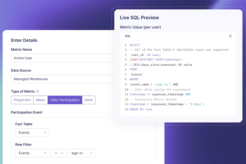
Historical trends are evidence, not a certificate
Plot several untreated periods when the data support it. Check whether the group gap was stable, whether measurement changed, and whether the chosen comparison tracks the business mechanisms you care about. One before period is enough for the arithmetic but offers little historical evidence for the identifying story.
A nonsignificant pretrend test does not prove parallel trends. Pretrend tests can have low power, so deviations large enough to matter may go undetected. Selecting specifications because they passed such a test can also distort subsequent inference.
Look at the size and uncertainty of plausible deviations, not only their p-values. Decide which departures would materially change the business conclusion. Keep the comparison-selection rationale and the diagnostics together so a reviewer can see how much the result depends on judgment.
Build data and uncertainty around the rollout unit
Distinguish a panel from repeated cross sections
A panel observes the same units over time. For an account-level panel, each row might represent one account in one week, with a stable identifier and consistently defined outcome.
Repeated cross sections observe different individuals in each period. Weekly cohorts of newly eligible accounts are an example. DiD can use either structure, but their data requirements and estimators differ. A series of average conversion rates does not tell the analyst which structure generated them.
Composition needs attention in both cases. A campaign may bring a different mix of accounts into the postlaunch cohort. A panel restricted to accounts present in every period may exclude churners, and treatment could affect who remains observed. Neither issue disappears by adding unit fixed effects.
Document enrollment, attrition, missing outcomes, and the population represented by each period. Do not silently turn missing data into zero outcomes or remove units based on behavior that treatment may influence.
Preserve windows, denominators, and source changes
Use complete and comparable outcome windows. If recent postlaunch accounts have only 2 days to activate while baseline accounts had 7, the period contrast mixes treatment with incomplete measurement.
Check the source events as well as the resulting rates. A renamed activation event or new identity-resolution rule can create a discontinuity exactly at rollout. A chart can look like a product effect because the release also changed what gets logged.
GrowthBook's metric examples distinguish user conversions from counts and revenue, which is useful when specifying the underlying data. Carry the same discipline into the observational dataset: identify the measured unit, aggregate events appropriately, and preserve a clear period field.
Do not substitute cumulative experiment snapshots for period-specific outcomes. GrowthBook's experiment time series shows cumulative results. A DiD dataset needs the actual outcome for each defined unit-period or cohort-period; differencing cumulative percentages generally does not recover it.
Audit the cohorts that straddle launch
Suppose the new flow launches on a Wednesday. An account enrolled on Monday may complete part of its 7-day activation window before launch and part afterward. Labeling every outcome recorded after Wednesday “treated” misclassifies its treatment history. Labeling the whole enrollment week “before” may also hide exposure.
Specify whether treatment is defined by eligibility date, actual availability, or another intervention rule. Then identify which cohorts have a clean treatment history under that definition. A prespecified transition period can help construct interpretable comparisons; removing inconvenient cohorts after seeing their outcomes is a different procedure.
Inspect individual source rows from both groups and both periods. A reviewer should be able to trace an account's market, eligibility timestamp, effective release timestamp, completed outcome window, and outcome value. Reconcile those rows with the totals in the four-cell table. This audit catches mistakes that a regression summary cannot explain: joining the wrong market identifier, using ingestion time instead of event time, or counting the same account in several enrollment cohorts.
Count independent rollout information honestly
If treatment changes at the market level, accounts within a market share treatment status and may share shocks. The same market observed in successive weeks can also have correlated outcomes. Treating every account-week as independent can make confidence intervals look much narrower than the design supports.
Plan inference around the treatment-assignment and error-dependence structure, often clustering by the rollout unit. The appropriate choice can be more complex when shocks operate across multiple levels. Cluster-robust standard errors address dependence under their assumptions; they do not remove differential confounding.
Millions of account rows spread across 2 markets do not become millions of independent rollout comparisons. With few treated or comparison clusters, familiar large-sample approximations can be unreliable. Small-sample adjustments, suitable bootstrap methods, or design-based approaches require their own justification. A bootstrap label is not a universal cure for a weak design.
The inference discussion in modern DiD methods emphasizes that few-cluster solutions rely on additional conditions. Check the number of independent treated and comparison units before committing to the study, not only after the point estimate looks promising.
If a future release can randomize at the account, organization, or market level, consider that option before defaulting to another observational comparison. GrowthBook's cluster experiment workflow addresses randomized group assignment with individual outcomes. That is a distinct design from fitting a clustered DiD model to nonrandom rollout dates.
Handle staggered launches without mixing incompatible comparisons
A single regression coefficient can hide different effects
Now suppose markets launch in different months. Early markets have several months of treatment history when later markets launch. The treatment may also work differently by market or become more effective as teams learn the new flow.
A conventional two-way fixed-effects regression includes unit and time effects plus a treatment indicator. In staggered settings, its coefficient can combine many simple comparisons. The timing decomposition of regression DiD makes that aggregation visible.
Some comparisons use already-treated units as controls for newly treated units. If the early units' treatment effect is still changing, their observed change includes treatment dynamics rather than only the untreated trend. The resulting coefficient can be difficult to interpret as the average effect your team intended to estimate.
This concern does not invalidate every fixed-effects model. It means that the simple 2-group, 2-period interpretation does not automatically carry over to many adoption dates and heterogeneous effects. Inspect the comparisons instead of assuming fixed effects make them suitable.
Estimate cohort-time effects that match the question
One approach is to define group-time treatment effects, written ATT(g,t): the average effect at calendar time t for units first treated in cohort g. The Callaway–Sant'Anna framework develops identification, estimation, and aggregation around these quantities, including settings where parallel trends is conditional on observed covariates.
A cohort-time approach makes the comparison explicit. For a given treatment cohort and period, suitable controls might be never-treated units or units not yet treated. Neither choice is automatically valid. Never-treated markets may differ systematically; not-yet-treated markets must still satisfy the relevant trend and anticipation assumptions.
The official group-time estimator reference exposes these choices, along with anticipation and panel settings. Review them deliberately. For example, software that balances a panel by dropping incomplete units can change the population being analyzed.
Conditional adjustment is also a design choice. Use covariates with a defensible pretreatment role when they make untreated changes more comparable. Controlling for postlaunch usage caused by the new flow can remove part of the effect or introduce selection bias. More covariates do not necessarily mean a more credible estimate.
Separate dynamic effects from changing cohort weights
An event study aligns outcomes by time since treatment. It can help describe whether the estimated effect differs on impact versus several periods later. But conventional lead-and-lag regressions can be contaminated by heterogeneous effects from other periods when treatment timing varies. Use a method appropriate to that structure.
Also check which cohorts contribute at each exposure age. Only early adopters may have 6 months of follow-up. A difference between month 1 and month 6 can reflect different cohort composition as well as treatment dynamics.
Aggregation should answer an explicit question. In a hypothetical same-horizon comparison, suppose 25% of treated accounts belong to a cohort with a 2-point effect, and 75% belong to a cohort with a 6-point effect. Account-size weighting gives 5 points; equal cohort weighting gives 4 points. Both calculations are correct, but they summarize different populations.
Report the weighting and support alongside the estimate. When every group has adopted, later effects may lack a suitable untreated comparison. A model can extrapolate beyond that support, but the result then depends on additional assumptions that should be visible.
Make the analysis useful in a rollout decision
Write a protocol before selecting the winning specification
A practical analysis plan should identify the treated population, rollout unit, effective treatment date, comparison pool, outcome scale, and horizon. It should explain why untreated changes are plausibly comparable and name the main ways that story could fail.
Record the estimator, aggregation weights, covariates, and inference method before inspecting a large collection of results. Specify which alternative windows or controls are planned sensitivity checks. Otherwise, choosing the most favorable comparison, launch date, and metric can turn an apparently rigorous analysis into a search for a positive number.
Keep a release-and-measurement log with the dataset. For the onboarding example, that includes campaign changes, sales training, product incidents, tracking deployments, and market-specific events. Reviewing that log with product and operations teams can reveal a competing explanation that is invisible in the regression output.
Ask how much counterfactual error changes the decision
Sensitivity analysis asks how conclusions change when the identifying assumptions weaken. The HonestDiD approach formalizes restrictions on departures from parallel trends and constructs inference under those restrictions. Its conclusions still depend on the restrictions being substantively appropriate.
For the illustrative 5-point estimate, ask whether a plausible differential untreated improvement could account for much of that gap. If a treated-only campaign could credibly explain several points, a narrow statistical interval around the DiD estimate does not resolve the attribution problem.
For a transparent hypothetical sensitivity calculation, suppose treated markets would have improved 4 points more than the comparison markets even without the flow. That violation contributes 4 points to the estimated contrast, leaving a 1-point treatment effect rather than 5. This is an assumption-based illustration, not an estimate of the campaign's impact. Its purpose is to make the identifying uncertainty tangible: reviewers can discuss whether a 4-point untreated differential is credible and whether a 1-point effect would justify the release.
Placebo dates, negative-control outcomes, alternative comparisons, and historical trend checks can expose problems. Passing them does not prove the counterfactual. Explain what each check could detect and what important violations it would miss.
Report what the evidence supports and improve the next design
A useful readout combines the effect estimate and interval with the target population, horizon, comparison rationale, diagnostics, sensitivity results, and remaining threats. Distinguish “the estimate remains positive under these assumptions” from an unconditional claim that the release caused the entire observed improvement.
For randomized experiments, GrowthBook's decision framework makes success criteria and target MDEs explicit. The transferable habit is to connect uncertainty to an agreed decision threshold. An observational DiD analysis also needs its identifying assumptions alongside that threshold.
GrowthBook's documented statistics engines analyze experiments; their presence does not make a nonrandom before-and-after comparison a native DiD estimate. Use appropriate external statistical methods for the observational design and keep its evidence separate from a randomized result.
When another release can preserve a randomized comparison, plan it prospectively. A warehouse-native experimentation workflow can reuse business metrics while assignment creates the comparison. When randomization remains unavailable, the next best improvement may be earlier baseline collection, cleaner rollout timing, more independent comparison units, or a better measurement contract.
DiD earns its value by making the missing counterfactual explicit. The final question is whether that counterfactual is credible enough for the decision you need to make.
Plan the next release comparison
When randomization is feasible, define the assignment unit and success metrics before rollout. Start a GrowthBook experiment using the data and outcomes your team already understands.
Get Started With GrowthBookRelated Articles
The same test statistic can support different conclusions when its degrees of freedom change.
You open an experiment report and see a t-statistic, a p-value, and a number labeled df. It might be 49, 118, or 19.48. That last value is not a typo. Degrees of freedom do not always equal the number of users minus 1, and they do not always come in whole numbers.
Degrees of freedom describe the independent variation available to a particular calculation or index the reference distribution used for inference. In familiar variance calculations, constraints explain them directly. In methods such as Welch's t-test, an approximation produces an effective value instead.
For experimentation, the useful question is specific: which calculation produced this df, and does that calculation match the data? Understanding that connection helps you spot wrong denominators, mismatched tests, and confidence intervals built from the wrong reference curve.
Start with the constraint behind n minus 1
Three observations, two freely varying deviations
Take a hypothetical sample of 3 measurements: 2, 4, and 6. Their mean is 4. Subtract that sample mean from each measurement and the deviations are -2, 0, and 2.
Those deviations sum to zero. They must: the mean was calculated from the same values. Once you know the mean and the first 2 deviations, the last deviation is determined. If the first 2 sum to -2, the last must be 2.
This is the intuition behind n - 1 degrees of freedom for the usual sample variance. There are n deviations but 1 independent linear constraint. Their possible patterns occupy n - 1 independent directions. You have not discarded a person or stopped using a measurement. All 3 values still contribute to the variance calculation.
You can see the arithmetic in this sample. Squaring the deviations gives 4, 0, and 4, for a total of 8. Divide by n - 1, which is 2, and the sample variance is 4. The sample standard deviation is its square root, or 2.
Why estimating the mean changes the denominator
The sample mean is fitted to the observed data. Deviations from that fitted mean tend to be smaller than deviations from the unknown population mean. For independent observations from the same distribution with finite variance, dividing their squared sum by n - 1 corrects the downward bias in the variance estimate.
The usual sample variance and one-sample t calculation therefore share the n - 1 quantity. This does not make the sample standard deviation itself exactly unbiased; taking the square root is a separate operation.
If your dataset is the entire finite population you want to describe, averaging squared deviations over n is a legitimate descriptive calculation. The denominator depends on the target. Estimating variation in a larger population is different from describing the values you already have.
Keep the intuition within its scope
“Independent observations minus fitted parameters” is useful for ordinary linear models, but it is not a universal df calculator. You must know what statistic is being calculated and what constraints or approximations apply.
Even a software parameter called ddof needs interpretation. The degrees-of-freedom adjustment in a standard-error calculation controls a variance denominator. It is not an instruction to use the same number as the reference df for every later test. A variance correction, a model's residual df, and a test's reference df are related concepts, not interchangeable labels.
See how df changes a statistical threshold
A t-statistic needs a reference curve
A t-statistic expresses an estimated difference relative to its estimated standard error. Its interpretation depends on the reference t distribution, whose shape is indexed by df. Low-df t distributions have heavier tails, reflecting uncertainty in the variance estimate under the model.
For a prespecified two-sided test at a 5% significance level, compare the absolute t-statistic with the appropriate 97.5th percentile. The t critical-value table gives approximately 2.776 at 4 df and 1.984 at 100 df.
Suppose two separate hypothetical analyses each produce t = 2.1. At 4 df, that value does not cross the 5% threshold. At 100 df, it does. The difference is not a judgment about the product feature. It follows from the reference distributions used to assess sampling uncertainty.
The reference distribution must itself be appropriate. Exact one-sample t inference assumes independent, normally distributed observations; large-sample approximations can cover broader settings. A small df does not automatically make a test invalid, but it gives you little protection against a poor distributional approximation. For highly skewed revenue measured on a handful of users, looking up the correct df is only one part of assessing the method.
Degrees of freedom are not the effect size
Larger df do not mean a bigger lift or a better variant. A tiny effect in a large sample can have high df. A large but imprecise effect in a small sample can have low df. You still need the effect's units, its interval, and a business threshold for deciding whether it matters.
Nor should you interpret df as statistical power. Power depends on the effect size you want to detect, variability, allocation, sample size, significance rule, and design. Use power analysis before launching an experiment to plan sensitivity. Reading a large df after the experiment does not replace that work.
Make small effects easier to detect
Degrees of freedom are only one part of uncertainty. Explore metric design and variance reduction techniques that can improve an experiment's sensitivity.
Explore Variance ReductionChoose the formula for the method you actually use
One sample, pairs, and pooled groups
For a one-sample t-test, n independent observations give n - 1 df. For a paired t-test, calculate a difference within each pair, then analyze those independent differences. With 30 complete pairs, the usual paired test has 29 df, not 59.
For the pooled two-sample t-test, the common variance estimate combines the two groups' variance information. Its df are nA + nB - 2. The test assumes equal population variances as well as independent groups. You should not select that formula merely because you have an A/B experiment.
| Calculation | Usual degrees of freedom | What must be counted correctly |
|---|---|---|
| One-sample t-test | n - 1 | Independent observations in the sample |
| Paired t-test | Number of complete pairs - 1 | Independent pairs, not both measurements separately |
| Pooled two-sample t-test | nA + nB - 2 | Independent group sizes and the common-variance assumption |
| Welch's two-sample t-test | Welch-Satterthwaite approximation | Each group's size and variance |
| Ordinary least-squares residual variance | n - rank(X) | Usable rows and independent columns of the design matrix |
| Chi-square independence test | (Rows - 1) × (Columns - 1) | The contingency table's category structure |
These are method-specific formulas, not options to try until a result becomes significant.
Welch can produce fractional df
Welch's t-test estimates each group's variance separately. Its reference degrees of freedom depend on how much each estimated variance contributes to uncertainty in the difference.
Consider a hypothetical revenue comparison with 20 independent units in group A and 100 in group B. The sample standard deviations are $20 and $5. For the absolute mean difference, the variance contributions are 20²/20 = 20 and 5²/100 = 0.25. Their sum is 20.25, giving a standard error of $4.50.
The Welch-Satterthwaite calculation is:
Here it gives approximately 19.48 df, even though there are 120 units in total. Most of the estimated uncertainty comes from the small, variable group A. Adding observations only to the already precise group B cannot remove that bottleneck.
Using 118 df because 20 + 100 - 2 = 118 would substitute the pooled method's assumptions. Rounding 19.48 up to 118 is not a harmless simplification. Let the chosen method calculate its df rather than overriding it from the total headcount.
Regression and count tables constrain different things
For ordinary least squares, residual df equal observations minus the design matrix's rank. With 100 usable observations, an intercept, and 2 nonredundant predictors, the rank is 3 and residual df are 97. Include the intercept in that count. Redundant predictor columns do not each add an independent fitted direction.
If the model fits an independent parameter for every usable observation, residual df can fall to zero. An exact fit then leaves no residual information for the usual error-variance estimate. Adding predictors until the observed data fit perfectly is not evidence that future outcomes will be predicted perfectly. A model's flexibility and its evidence for uncertainty are different things.
Ordinary one-way ANOVA illustrates another reason to read the label carefully: its F reference distribution has 2 df values. For k groups and N independent observations, the between-group and error degrees of freedom are k - 1 and N - k. A hypothetical comparison of 3 variants across 90 observations has F reference df of 2 and 87. The corrected total is 89, which equals their sum. Reporting only “df = 89” would omit the information needed to identify that F distribution. These formulas belong to the ordinary one-way model with its variance assumptions; they are not a recipe for every repeated-measures or unequal-variance ANOVA.
A chi-square test of independence uses a different structure. A 2-dimensional contingency table has (rows - 1) × (columns - 1) df. A 2-by-2 variant-by-conversion table has 1 df, whether it contains 200 users or 200,000. More traffic improves precision; it does not change the number of category relationships tested.
This is why df cannot serve as a universal substitute for sample size. Its meaning comes from the statistic and model.
Check the experimental unit before trusting a large df
Repeated events do not create independent users
Suppose you assign 1,000 users to a new experience and record 50,000 pageviews. A user-level treatment comparison does not gain 49,999 df just because the event table has that many rows. The same person's repeated events can be correlated.
Aggregate outcomes or model their dependence in a way that matches the design. A revenue-per-user metric, for example, can sum each user's eligible purchases over a fixed window before comparing groups. Explicit metric and Fact Table definitions help make that relationship between event rows and analyzed units inspectable.
Group assignment creates another case. If treatment is assigned to organizations, employees within an organization share an assignment and may influence one another. A cluster experiment needs inference that accounts for that structure. Plugging the number of employees into an ordinary independent-observation formula does not make the dependencies disappear.
Missingness changes the usable data
Check the data used for the specific metric, not only the experiment's top-line traffic count. Different metrics can have different valid windows, available measurements, or exclusions. In a paired analysis, incomplete pairs can reduce the number of usable differences.
That numerical reduction is only part of the issue. If treatment influences whether an outcome is observed, complete-case analysis can change who gets compared. A plausible df cannot tell you whether the missingness mechanism introduced bias.
Investigate a surprising value by tracing the inputs: which observations survived, what identifier defined an independent unit, what model was fitted, and whether the output uses an approximation. Treat df as a diagnostic clue rather than a quality certificate.
Also distinguish statistical df from the phrase “researcher degrees of freedom.” The latter refers to choices such as which metric, segment, exclusion, or analysis to report. Exploring those choices after seeing results can change the interpretation of evidence. It does not change the arithmetic identity n - 1 for a particular sample variance. Record the planned analysis and label exploratory follow-ups so a reader can distinguish the two issues.
Report the method behind the number
Keep df attached to the estimate and interval
A useful report names the test, the usable group sizes or pair count, the estimated effect, its standard error or interval, and the reference df when relevant. “Welch's t-test, df = 19.48” tells a reviewer more than “t-test, 120 observations.” Neither replaces an explanation of the experiment's assignment and measurement rules.
When reproducing a result, preserve the method's assumptions and software settings. A pooled t-test, a Welch test, and a model with clustered standard errors can analyze similar-looking columns while making different inferential calculations. Matching the displayed row count is not enough to reproduce the p-value.
GrowthBook's frequentist statistical calculations use a t reference distribution with degrees of freedom estimated through the Welch-Satterthwaite approximation. Its statistics overview also distinguishes frequentist and Bayesian engines. A df formula from one approach should not be inserted into the interpretation of another approach's output.
Resolve design problems before chasing precision
Before your next experiment, verify the unit of assignment and analysis, define the metric window, and choose the estimator and decision rule. Those decisions determine what information the analysis can use.
The stopping rule matters separately. A correct df does not authorize repeatedly inspecting a fixed-horizon p-value and stopping when it passes. If you need continuous decision-making, use a suitable method such as GrowthBook's frequentist sequential testing within its documented scope.
You rarely need to calculate degrees of freedom by hand in a production experiment. You do need to recognize when the reported value reflects the wrong test or the wrong independent unit. Start with the design, follow the calculation, and read the effect with its uncertainty. The df will then be an interpretable part of the result.
Build a test you can explain
Define your experiment's metrics and data source in GrowthBook, then review the treatment effect with its uncertainty and documented analysis method.
Get Started With GrowthBookChoosing where a variant runs is only the first architecture decision.
A checkout experiment can make its decision on the server, render in the browser, and measure purchases in a warehouse. Calling it “server-side” tells you little about whether the person received the assigned experience or whether their purchase joined to the right group.
Server-side testing evaluates or executes treatment logic in a backend service before returning its result. Client-side testing evaluates or applies treatment logic in the user's browser or application. Both can support randomized experiments. Both can fail through inconsistent identity, incorrect exposure events, or measurement that changes with the treatment.
The useful comparison starts with the change you want to test. A ranking algorithm belongs near the service that runs it. A browser interaction may belong in the application that renders it. Then work through the entire path from assignment to outcome, including the cache, navigation, and login transitions between them.
Separate the experiment's four locations
Assignment is different from treatment delivery
Assignment selects a variant for an eligible unit. Delivery makes the application behave according to that variant. They often happen together, but they do not have to.
For example, an edge worker can select a layout and a browser can render it. A backend can select a recommendation algorithm and return its results as JSON. A browser can select a button label without involving the server in that decision. The same statistical question can sit behind any of these implementations.
Describe the architecture with verbs: who assigns, who executes, who records exposure, and who computes the metric. That description is more useful than the label “full stack.” GrowthBook supports feature flags on the client and server, but you still choose which code consumes each flag and which system supplies the outcomes.
Exposure and analysis can live elsewhere
An exposure record should represent the experiment event your analysis is designed to use. An SDK evaluation callback tells you that an evaluation enrolled a user; it is not proof that the corresponding screen was visible or that a response reached a person.
If you evaluate a checkout flag during application startup but never use its value, the callback can precede any relevant treatment. If you log after the page finishes loading, a slower treatment can lose more events before the logger runs. Both mistakes change what the experiment population means.
Analysis has another location. With warehouse metric definitions, you can join assignment records to purchases or retention data already collected in your own data system. Running the branch on a server does not mean the server SDK has automatically captured or analyzed those outcomes.
Compare complete delivery paths
| Decision | Browser implementation | Server implementation | Hybrid implementation |
|---|---|---|---|
| Where treatment executes | Browser UI or application behavior | Backend logic, API behavior, or rendered response | Different parts execute in different runtimes |
| Main implementation dependency | Frontend code or an eligible visual change | Backend deployment and service integration | Shared identity and explicit ownership across layers |
| First-render concern | Apply the intended experience before visible replacement | Return the intended response without avoidable delays | Preserve the server result during hydration |
| Measurement concern | Blocked, delayed, or missing client events | Join server assignment to actual delivery and outcomes | Avoid duplicate or contradictory exposure records |
| Cache concern | Stale configuration or application state | Variant-specific responses shared incorrectly | Cache keys and browser state disagree |
These are engineering tradeoffs, not a universal speed ranking. A browser SDK can evaluate configuration already available locally. A server can add network waits if it fetches configuration on the request path. Measure the path you actually deploy.
Put the treatment where it can be implemented faithfully
Use the browser for changes the browser owns
Client-side testing suits interactions such as showing a different onboarding step, changing a filter interface, or selecting a message inside a web application. A developer can implement the variant directly in application code. A visual editing tool is another route for supported page changes, but client-side testing is not limited to editing the DOM after a page loads.
That distinction matters when teams compare ownership. Some changes can be authored by a growth team in a visual workflow; others require frontend engineering even though they run in the browser. The deployment and review process follows the implementation, not the statistical label.
Browser execution can create a visible replacement if the original content paints before the variant is applied. Hiding the entire page until configuration arrives can create a different problem: a long blank screen when the dependency is slow. Prefer an explicit rendering and fallback strategy over assuming every client-side test must flicker or that an anti-flicker snippet has no cost.
Use the server for backend behavior and controlled responses
Server-side testing fits a pricing calculation, search ranker, checkout service, recommendation pipeline, or response assembled before it reaches the browser. You can keep service credentials and confidential implementation details in that environment.
That benefit has a boundary. If you serialize sensitive rules, identifiers, or secrets into HTML or a browser configuration payload, their earlier evaluation on the server does not make the delivered data confidential. Review exactly what crosses the boundary.
Keep authorization independent of experimentation. A flag can select an experience for an already authorized user; it should not be the only check deciding whether that user can access a protected resource. Apply permission validation on requests regardless of the assigned variant. A client can alter browser state and requests, so browser-visible eligibility is especially unsuitable as a security boundary.
Measure performance instead of promising it
Server rendering can avoid a particular after-paint replacement, but it can also increase response time if the new branch is expensive. Client rendering can avoid a backend change while adding JavaScript work or delaying interactivity. Edge execution can shorten one network path while introducing cache and configuration-update concerns.
Compare the control and treatment on the experience people receive. Core Web Vitals distinguish loading, interaction responsiveness, and layout stability. Pair those measures with relevant backend latency and error metrics. A low flag-evaluation time does not describe the cost of the treatment, the configuration fetch, or the event pipeline.
Define fallback behavior before launch. If configuration is unavailable, decide which existing behavior remains appropriate, how the failure is observed, and whether that request belongs in the experiment analysis. Quietly mixing fallback users into an assigned treatment can dilute or distort the comparison.
Choose the smallest complete treatment
Consider 2 hypothetical checkout ideas. One changes the explanation beside a shipping option; the other changes the shipping-price calculation. The first can live in the frontend if that application already has the necessary context. The second belongs with the authoritative calculation so the displayed amount and the charged amount agree.
Combining both into one treatment may be a reasonable product decision, but it answers a broader question. If the experiment wins, you cannot attribute the change to the explanatory copy alone. Write down what differs across arms before deciding which team or runtime will implement it.
For a first integration, keep unrelated behavior identical. Use the existing purchase event and metric definition when they already represent the outcome you need. Changing rendering, pricing, identity and analytics together makes a surprising result harder to diagnose. A small experiment should still include the whole assignment-to-outcome path; small does not mean skipping instrumentation review.
Plan flags across your stack
Extend the architecture decision into ownership, lifecycle management, and production review. Use the feature flag guide to plan how flags will operate as your program grows.
Read the Feature Flag Guide
Keep identity and delivered variants consistent
Scope user attributes to the request
A shared configuration client is useful on a server. Shared mutable user attributes are a different matter. If one request replaces a global user's attributes while another request is evaluating a flag, users can receive each other's targeting context.
The current GrowthBook Node.js SDK supports a shared GrowthBookClient with a user context passed to evaluation, or a scoped instance for that context. Keep the authenticated or anonymous identifier in the request's scope. Do not use an arbitrary user-supplied identifier as authentication merely because it is convenient for experimentation.
Choose the randomization unit deliberately. A user-level experiment needs a stable user identifier; an account-level workflow may need an account identifier. Requests and pageviews are usually repeated measurements of those units, not new independent participants. Every service participating in the same treatment needs the agreed unit and identifier representation.
Treat login and configuration changes as design events
If a visitor is assigned using an anonymous identifier and switches to a different identifier after login, they can receive another variant. That is a design problem to resolve, not a reason to overwrite the old event history.
Document the identity transition, warehouse join, and intended assignment persistence. Sticky bucketing persists assignments for supported workflows; it is distinct from ordinary deterministic hashing with unchanged inputs. It does not make arbitrary identity changes or incompatible configurations equivalent.
For cross-runtime parity, verify the same experiment definition, hash attribute and its type, seed, hashing version, targeting context, and applicable rules. A string identifier and a numeric identifier should not be assumed interchangeable. Matching a few sample users is a useful diagnostic; it is not proof that every production context is equivalent.
Configuration versions also belong in the handoff. A browser tab can hold yesterday's payload while a server uses a newer one. Decide how a running experiment handles configuration refreshes and which changes require a new phase or a new experiment. Record enough metadata to diagnose disagreements without sending confidential configuration into public events.
Treat an SDK upgrade as a change to verify, too. The official JavaScript SDK changelog identifies behavior changes across versions, including attribute-type handling. Preserve your lockfile and run representative targeting and assignment checks when upgrading. A matching experiment key alone does not establish that two different SDK versions and payloads make equivalent decisions.
Make caching and hydration part of the experiment
A shared cache that keys only on URL can return the first cached variant to users assigned elsewhere. You need a cache design that preserves the intended partition without leaking personalized content between users.
Cache-Control directives distinguish private responses and storage restrictions. The Vary header describes request header fields used to select a response. Neither is a substitute for checking the actual CDN and framework cache configuration. A variant cookie does not help if the relevant cache ignores it.
With server-rendered React, the initial browser render should match the server HTML. Hydration expects matching content; changing the assigned variant on the client can create mismatches as well as a compromised treatment. Pass only the public state the browser needs, preserve the initial decision, and test navigation and login transitions separately.
Verify SDK parity before wiring production delivery
Start with a local fixture and explicit prerequisites
The following fixture compares the Node shared-client API with the GrowthBook class used in browser integrations. It runs both inside Node against synthetic configuration. It does not render a page, contact GrowthBook, send analytics, or implement production identity.
Use a currently maintained Node.js release and an empty local directory. The callback context used below requires GrowthBook SDK 1.7.0 or later; this example pins version 2.0.0. Install the package, keep the lockfile, and inspect the resolved version before continuing:
If installation fails, fix that prerequisite before running the fixture. Do not replace the SDK with a homemade hash and treat that as a check of the SDK's behavior. The browser JavaScript SDK documents the GrowthBook class, payload initialization, and tracking callback used here.
Save this as parity.mjs. The payload is an illustrative 50/50 experiment, not a production SDK connection or a CMS-created experiment:
The callback's objects are local diagnostic records defined by this example. They are not a transport contract, and putting an object in this array does not insert an exposure into your analytics system.
Run the check and interpret its limits
Use strict assertions to fail visibly when these invariants do not hold. Check syntax, then execute the file:
If the assertions pass, the script prints the PASS line. An import error means the dependency is missing or cannot be resolved. An assertion failure requires inspection of the installed SDK, payload, identifiers, and context; do not change an expected value simply to silence it.
The fixture checks equal values for these synthetic identifiers, repeatability within a scoped context, both values appearing, and identifier-shaped callback diagnostics. It does not establish a precise 50/50 sample split. It also does not prove request concurrency isolation, browser compatibility, actual rendering, or production identity correctness. Add those checks in your application's environment.
Replace the fixture boundary deliberately
For a real application, initialize configuration using the documented SDK connection and its failure-handling path. Supply identity from your application rather than the synthetic loop. Consume the selected value at the point that controls the treatment, then verify the response or UI actually follows it.
Browser integration additionally needs the application's module bundler or supported script integration, configuration readiness, and rendering lifecycle. A Node console run cannot verify those. If you use React, follow the React SDK integration rather than assuming the fixture provides a provider, hooks, or hydration handoff.
Finally, connect the documented callback or supported tracking integration to your real collection system. Map its experiment key, variation key, evaluation-time identity and timestamps to your agreed schema. Keep the mapping and retry behavior inspectable; do not copy the diagnostic array into a production event pipeline and assume attribution is complete.
Validate delivery and measurement before interpreting lift
Trace one unit through the entire path
For an isolated QA user, capture the input identifier, configuration version, selected value, delivered response, exposure record, and eventual outcome join. Repeat for both branches, a returning visitor, a login transition, and a missing-configuration fallback. Use a QA environment or isolated event sink so these checks do not create production experiment outcomes.
Test the real cache path. Make requests as different units, revisit the same unit, and inspect whether cache hits preserve the intended behavior. Test server-rendered content before JavaScript runs, after hydration, and after client-side navigation. A successful flag evaluation alongside the wrong UI is a failed experiment integration.
Include failure cases rather than only a successful page load. Delay configuration, drop the analytics request in an isolated test, and open an old tab after publishing a new QA payload. Check whether each case uses the intended fallback, keeps the correct identity, and leaves enough evidence to explain its inclusion or exclusion from analysis.
For a backend service, exercise overlapping requests from different QA users while inspecting the selected values and evaluation contexts. The sequential fixture above cannot reveal a race in your own middleware. For a browser, test a slow device and a failed script request, not just a fast development laptop. These checks target the actual ways a delivery path can diverge from its assignment record.
Write the expected failure behavior before running the checks. If an event does not arrive, the acceptable result is an observable gap with a documented handling rule, not a fabricated conversion or a silent reassignment. Keep operational recovery separate from any decision to change the experiment's analytical population.
Evaluate only where the value is relevant. GrowthBook's feature rule types distinguish targeted value delivery from an experiment rule. A percentage release is not automatically a measured A/B comparison, and a callback for a value that was never consumed does not demonstrate treatment exposure.
Reconcile collection instead of trusting one callback
Server assignment can reduce reliance on a browser for one event, but client outcomes can still be missing because of blockers, consent state, navigation, or transport failure. Server events can also fail through queues, retries, schema errors, or joins. Decide what is collected and eligible under your actual consent and measurement policy, then test that implementation symmetrically across arms.
Beacon-style analytics delivery can help with page transitions, but a successful enqueue is not proof of warehouse receipt. Reconcile callback or server logs with received events and the analyzed population. Preserve meaningful timestamps and define how duplicates are handled at the randomization unit.
Look for variant-specific loss. If treatment slows the page and its exposure is logged only after an animation completes, the retained treatment cohort can look unusually engaged. Moving assignment to the server does not repair that later selection. Record the relevant eligibility event consistently and inspect where users disappear between stages.
Consider a hypothetical collection audit with 1,000 known eligible QA units in each arm and 120 purchasers in each. Both full cohorts convert at 12%. Now suppose the exposure table retains only 900 control units and 980 treatment units, while retaining every purchaser. An analysis restricted to those recorded exposures reports 13.33% versus 12.24%. The apparent difference comes from the denominator loss, not the treatment.
In production, you cannot assume you know the missing units' outcomes as you do in this constructed example. That is why reconciliation starts with the eligibility and collection definitions, rather than repairing counts until a result looks plausible. Find the stage that lost records and assess whether the original comparison remains recoverable. More sophisticated statistics cannot restore an unidentified missing cohort.
Keep the analysis and rollback decision explicit
GrowthBook's data quality checks include sample ratio mismatch and multiple exposures. Use them alongside raw event reconciliation. Passing a traffic-split check does not prove every assigned user received the right treatment, and balanced counts do not reveal all symmetric instrumentation errors.
Before the experiment starts, record the primary metric, observation window, guardrails, sample-size or duration plan, statistical method, and decision rule. Server and client delivery do not have different laws of inference. A larger event count still does not replace independent users or accounts, and repeatedly checking a fixed-horizon result still needs an appropriate decision procedure.
If you migrate an existing experiment from browser to server delivery, document the handoff before combining results. A new identity source or exposure definition can change the analyzed population even when the product treatment appears identical. Preserve the old and new collection definitions, compare them in an isolated environment, and decide whether a separate phase or a new experiment is needed.
An A/A integration check can help uncover allocation, rendering, or telemetry differences when both arms deliver the same behavior. It does not prove the absence of bias because the result is nonsignificant. Combine that diagnostic with known QA users, raw event comparisons, and code review. Check that temporary parallel collection does not cause the same assignment or purchase to be counted twice after the handoff.
Assign an owner to the rollback path as well as the launch path. Verify which configuration change restores the intended default, how cached configuration updates, and what happens to users already assigned. After a decision, preserve the experiment record and remove obsolete branches through normal engineering review.
The architecture is ready when the unit, delivered experience, and measured outcome tell the same story. Choose the runtime that can implement the treatment faithfully, then make that full path reviewable before interpreting its lift.
Build a measurable release path
Connect your application, define the outcomes that matter, and review assignment and data quality before using an experiment result to guide a release.
Get Started With GrowthBook
A rollout can create useful evidence even when you cannot randomize users. The comparison still has to earn a causal interpretation.
Your team introduces a new onboarding process in one market because its support team is ready first. Activation improves. That is encouraging, but the market also received a new acquisition campaign. A before-and-after chart cannot tell you how much improvement came from onboarding, the campaign, or changes that would have happened anyway.
A quasi-experiment uses a nonrandom assignment process and an explicit comparison strategy to estimate an intervention's effect. The comparison might come from another market, an eligibility cutoff, a policy rule, or a carefully modeled historical pattern. Its credibility depends on why that comparison represents what would have happened without the intervention.
This guide organizes the main designs around those opportunities. You'll learn which rollout situations support each design, what effects they can estimate, and which assumptions remain vulnerable even when a result looks statistically precise.
Identify the assignment mechanism before choosing a design
Quasi-experimental is a family of approaches
Definitions differ across fields. Some researchers use the label broadly for intervention evaluations without random allocation. Others reserve it for designs that exploit plausibly external variation in treatment. The practical question is the same: what makes the treated and comparison outcomes informative about a counterfactual?
The official guidance on quasi-experimental product evaluation describes several approaches and emphasizes the difficulty of choosing a comparison group. A label alone does not resolve that difficulty. Comparing users who voluntarily adopt a feature with users who ignore it may primarily measure motivation, need, or product familiarity.
An uncontrolled before-and-after study is especially weak when trends or other changes can explain the difference. Some taxonomies call this pre-experimental; others include it among weaker quasi-experimental designs. Describe the actual comparison instead of letting terminology imply more protection than the study provides. Design improvements for non-equivalent groups and time series help make those differences visible.
Group and time assignment can still be randomized
An experiment does not become quasi-experimental because you assign organizations instead of individual people. Randomly allocating organizations produces a cluster-randomized experiment. Randomly allocating eligible time blocks can produce a randomized switchback design, although carryover and time dependence need attention.
Conversely, assigning regions according to commercial priorities remains nonrandom even if the regions have similar population sizes. “Geographic” describes the unit, not the identification strategy.
GrowthBook's cluster experiment workflow supports group-level randomization with appropriately configured individual-level outcomes. Before accepting that randomization is impossible, investigate whether a different unit or a narrower eligible population would make it feasible. That is a design decision, not a reason to pretend account-level assignment creates independent user-level observations.
Specify the effect before opening the results
Write down the intervention, eligible population, assignment unit, start time, outcome window, and effect you need. “Did onboarding work?” is too vague. “How did offering the new onboarding process affect 28-day activation among eligible accounts in the first rollout market?” identifies a clearer target.
Distinguish an offer from actual adoption. Adoption may depend on a user's motivation, which also affects activation. Restricting the analysis to adopters after launch can destroy the comparison you intended to study.
In a randomized implementation, experiment configuration makes the assignment attribute, hypothesis, and variation setup explicit. Carry the same discipline into a quasi-experimental protocol, while recognizing that documentation does not make a nonrandom assignment rule ignorable.
Use rollout timing to construct a credible comparison
Controlled before-and-after designs compare changes
Suppose a hypothetical product rollout changes 28-day activation as follows. The outcome definition and enrollment windows are the same in both markets.
| Market | Before rollout | After rollout | Change |
|---|---|---|---|
| First rollout market | 60% | 68% | +8 percentage points |
| Comparison market | 58% | 62% | +4 percentage points |
The treated market improved by 8 points, but the comparison market improved by 4. A difference-in-differences calculation subtracts those changes: (68 - 60) - (62 - 58) = 4 percentage points.
The corresponding counterfactual for the treated market is 64%: its original 60% plus the comparison market's 4-point change. The estimated effect is 68% minus 64%. This is different from attributing the entire 8-point rise to the rollout.
The difference-in-differences identification argument requires that the groups' untreated outcomes would have followed parallel changes over the relevant period. Their baseline levels can differ. A simultaneous campaign confined to the rollout market threatens that argument because its effect enters the same 4-point estimate.
Inspect several pre-intervention periods and understand how rollout priority was chosen. A non-significant pretrend test does not prove the assumption; limited data may simply fail to reveal an important difference. Stable metric definitions and denominators are also necessary, since a new activation event or eligibility rule can manufacture an apparent change.
Staggered adoption needs explicit comparisons
When markets adopt in different months, “not treated yet” and “already treated” are different states. An already treated market can have an evolving treatment effect, making it an inappropriate stand-in for an untreated outcome.
Do not default to a single two-way fixed effects coefficient without understanding its comparisons. With heterogeneous or changing effects, it can mix effects that do not match the decision you want to make. Group-time treatment effect methods make treatment cohorts and comparison choices explicit.
For a product team, the operational task is to preserve adoption dates, eligibility, and untreated comparison periods before the rollout spreads. Once every market adopts, later effects may lack a credible untreated comparison. More post-rollout rows do not recreate that missing design element.
Interrupted time series uses the intervention date
An interrupted time series, or ITS, models the outcome trajectory before a known intervention and asks whether the subsequent level or slope departs from that trajectory. It is more informative than comparing two averages when a trend was already underway.
Consider a mandatory checkout change released everywhere on the same day. A daily series could assess an immediate discontinuity, a gradual slope change, or a delayed effect. Choose the expected pattern before searching for the most favorable model. The ITS tutorial and its updated materials address seasonality, autocorrelation, and concurrent events that complicate this analysis.
An interruption still needs a defensible counterfactual. If a holiday promotion begins on release day, an observed jump cannot distinguish the two changes without further information. An unaffected comparison series can strengthen the design when it shares relevant shocks, but a series touched by the same checkout change cannot serve that role.
Strengthen the design first
Review experiment-design mistakes, metric choices, and long-term impact in this session with Ronny Kohavi and Luke Sonnet before committing to a rollout comparison.
Explore Experiment DesignUse cutoffs and external rules without overstating their reach
Regression discontinuity identifies effects near a threshold
A regression discontinuity design, or RDD, can be useful when a pre-existing numerical rule determines eligibility. Imagine a hypothetical service offering proactive onboarding support to accounts with a risk score of at least 70. Accounts just above and below 70 may provide a useful local comparison if other determinants of activation change smoothly at the threshold.
The local cutoff identification argument does not require all high-risk and low-risk accounts to be comparable. It concerns the limit near the cutoff. The resulting effect should not automatically be generalized to accounts with scores of 20 or 95.
Check whether teams can manipulate the score or override eligibility. Also check whether the threshold triggers another intervention, such as a pricing change. If several benefits change at 70, the design may identify the effect of that bundle rather than onboarding support alone.
Implementation requires a defensible neighborhood and functional form. A raw difference between broad score bands is not the same as estimating a discontinuity. Local polynomial RD tools provide estimation, bandwidth selection, plotting, and bias-corrected inference; they cannot establish that the eligibility rule was uncompromised.
Fuzzy eligibility changes treatment probability
In a sharp design, the threshold determines treatment. In a fuzzy design, it changes the probability of treatment because some eligible accounts decline support or some ineligible accounts receive an exception.
Suppose, purely as a numerical illustration, fitted adoption probability jumps from 20% to 80% at the cutoff while fitted activation jumps from 63% to 69%. The ratio is 0.06 / 0.60 = 0.10, or 10 percentage points. Interpreting that ratio as a treatment effect requires additional instrumental-variable assumptions, including that eligibility affects activation only through the treatment and that treatment uptake moves in the required direction.
Those assumptions matter more than the attractive arithmetic. The effect concerns accounts whose treatment changes because of eligibility near the threshold. It is not automatically the effect for every account that used support.
Natural experiments need an assignment story
A natural experiment exploits an externally determined event or rule that generates useful treatment variation. The event is not necessarily a literal disaster or a sudden policy change. What matters is why its assignment is plausibly unrelated to the otherwise expected outcome, within the proposed comparison.
An instrumental-variable design can use such variation to study adoption. But an instrument must affect treatment, be suitably independent of outcome determinants, and satisfy an exclusion argument. Instrumental-variable assumptions and local effects explain why a predictor of adoption is not automatically a valid instrument.
For example, a support-team capacity rule may change whether an account receives onboarding. If that capacity also changes response times for unrelated support requests, the rule can affect activation through another path. Calling the variation external does not remove that problem. Preserve the operational records needed to examine those paths before staff assignments or exceptions are forgotten.
Construct comparison groups without hiding selection
Synthetic controls combine untreated units
When one market receives an intervention, a synthetic control can combine other markets into a weighted comparison chosen to resemble its pre-intervention trajectory and relevant predictors. It can be useful when no single market is a convincing comparison.
In a hypothetical illustration, weights of 60% and 40% on donor outcomes of 24 and 29 produce a synthetic outcome of 26. If the treated outcome is 30, the post-intervention gap is 4 outcome units. That gap becomes a causal estimate only if the donor construction and counterfactual assumptions are credible.
The feasibility requirements for synthetic controls include the availability of suitable donors and informative pre-intervention data. Donors affected by the intervention, related campaigns, or spillovers can contaminate the comparison. Good historical fit is useful evidence, but it does not guarantee that the treated market avoided a unique post-intervention shock.
Choose donors and fitting decisions without optimizing the desired post-intervention result. Compare alternative defensible donor pools and examine placebo analyses, while recognizing that a small, unusual donor set limits what those comparisons can establish.
Matching and weighting depend on measured information
Matching can align treated and comparison accounts on recorded characteristics. Weighting can reweight observations toward a specified population. These approaches may improve a non-equivalent-group design, but balance on available columns does not establish balance on unmeasured intent or readiness.
The unconfoundedness and overlap requirements are central to causal interpretations based on measured adjustment. If every enterprise account receives onboarding and no comparable enterprise account goes untreated, a model may be extrapolating rather than making a supported comparison.
Use pre-treatment variables appropriate to the causal question. Do not adjust for completed onboarding steps when those steps are part of how the intervention changes activation. That can remove part of the effect or introduce selection bias. Treat the choice of adjustment variables as a design decision, not an automatic instruction to include every warehouse field.
Let the assignment process narrow the candidates
| Available variation | Candidate design | Main question to resolve |
|---|---|---|
| Some markets change while others remain untreated | Controlled before-and-after or DiD | Would untreated outcomes have changed similarly? |
| A known date interrupts a sufficiently informative series | ITS, preferably with a suitable control series | Could another event or trend explain the interruption? |
| Eligibility changes at a numerical threshold | Sharp or fuzzy RDD | Are potential outcomes continuous and the rule unmanipulated? |
| An external rule changes treatment uptake | Natural experiment or IV | Does the rule affect the outcome through another path? |
| One treated unit has suitable unaffected donors | Synthetic control | Can the donors support a credible post-intervention counterfactual? |
If none of these arguments fits, a descriptive comparison may still be useful. Report it as descriptive rather than converting it into a causal claim through a more complicated model.
Audit threats that precise estimates can conceal
Keep population and exposure definitions stable
An activation rate can rise because activation improved or because the analyzed accounts changed. Record who was eligible at each date, who entered the data, and how incomplete outcome windows were handled. A later cohort with only 7 days of follow-up should not be compared with an earlier cohort's completed 28-day outcome.
Differential attrition creates another problem. If the intervention changes whether accounts remain observable, complete-case analysis can compare selected survivors. Similarly, filtering to users who revisit can condition on behavior caused by treatment. Count definitions and exclusions should follow the question, not the apparent direction of the result.
Also distinguish assigned availability from actual exposure. A rollout date does not mean every account encountered the new process that day. A per-protocol question about adoption needs its own assumptions; it cannot quietly replace an offer-based question after the analysis begins.
Trace spillovers, anticipation, and shared shocks
Markets can affect one another through referrals, shared sales teams, supply constraints, or users crossing boundaries. An untreated region may therefore receive part of the treatment's effect. A comparison that is administratively untreated is not necessarily causally unaffected.
People may also change behavior before the official launch because of an announcement or training. Decide whether the treatment includes that anticipation period and adjust the protocol accordingly. The date in the release calendar may be too late to define the intervention's true start.
For randomized work, GrowthBook's data quality checks surface issues such as sample ratio mismatch and multiple exposures. Those checks support an experiment's data review; they do not test the parallel trends, exclusion, or continuity assumptions of a quasi-experiment.
Match uncertainty to the source of variation
Thousands of user rows from one treated region do not create thousands of independently treated regions. Shared regional shocks and repeated measurements can make row-level standard errors misleading. The inference method needs to reflect the unit and time structure that generate the treatment comparison.
Few treated or comparison units are particularly challenging. Cluster-robust calculations, resampling, or placebo procedures have design-specific requirements; none creates independent information that was absent from the rollout. Report those limits alongside the interval instead of hiding them behind a large event count.
A falsification check should challenge a particular explanation. For example, a rollout should not change an outcome measured before any announcement or exposure. An apparent effect there can reveal a timing problem, selection, or model failure. A negative-control outcome can be useful when it shares the suspected confounding process but cannot plausibly respond to treatment. The logic of falsification testing helps distinguish that exercise from simply adding more favorable outcome charts.
Passing a check is weaker evidence than failing a well-chosen one. An unaffected outcome may not share the relevant confounder, and a placebo test may have little power. Explain why the check would reveal the threat you care about, rather than treating a collection of non-significant tests as certification.
Statistical precision also addresses a different question from identification. A narrow interval under a misspecified counterfactual can be precisely wrong. The interpretation of experiment results should keep uncertainty and data quality visible, while a quasi-experimental review must additionally evaluate the assumptions creating its comparison.
Write a protocol that can survive the rollout review
Record the causal argument before estimating the effect
A useful protocol begins with a decision: what rollout choice will this evidence inform, and what magnitude would matter? Then state the treatment version, target population, assignment mechanism, counterfactual, outcome scale, observation window, and primary analysis.
Add a threat-specific diagnostic plan. For a cutoff, inspect the assignment rule, score distribution, and other changes at the threshold. For a timed rollout, investigate pretrends, announcements, concurrent campaigns, and comparison-group exposure. Choose checks because they challenge the causal argument, not because they are easy to pass.
State what would change the conclusion. A missing historical period, an unexplained composition break, or a coincident market-specific campaign might downgrade the analysis to descriptive evidence. This makes the review useful even when the preferred causal interpretation fails.
Preserve operational evidence while the rollout is happening. Keep the original eligibility rule, announcement and deployment dates, exception log, support-capacity changes, and a record of campaigns affecting each comparison unit. Save the version of the score used for cutoff assignment rather than a later score updated after treatment. Historical outcomes alone cannot reconstruct those decisions reliably.
For the onboarding example, an audit-ready record might say: the offer began on a specified date; eligibility used account status recorded beforehand; accounts received a completed 28-day window; the comparison market retained its original process; and the concurrent campaign was either separately identified or acknowledged as unresolved. Each statement answers a concrete design question. A table containing only account IDs, a treatment flag, and activation cannot answer them all.
Report the scope and alternatives with the estimate
Share the estimate with its units, uncertainty, target population, comparison, and identifying assumptions. Separate prespecified analyses from sensitivity checks and later exploration. A result near an eligibility cutoff, an effect on treated markets, and an effect for instrument-induced adopters are different answers.
When several defensible specifications agree, explain what they share. Agreement is less reassuring if every specification assumes away the same unmeasured campaign. When results differ, show which assumption, window, or population change drives the difference rather than selecting the most favorable estimate.
Keep transport to the next rollout separate from identification of the first effect. A result for accounts near a risk threshold may not predict what happens when support is offered to everyone. Wider deployment can change staff capacity, user composition, or interactions between accounts. Even a credible local estimate may therefore support a staged follow-up rather than a universal rollout decision.
Treat that limitation as useful information for planning. Name which accounts and operational conditions the evidence covers, which extension is uncertain, and what additional comparison would reduce that uncertainty. This gives the next experiment a specific job instead of repeating the same broad question with another model.
Preserve opportunities for randomized evidence
Operational constraints may leave room for a randomized subpopulation, cluster assignment, or delayed release. A planned A/B design can sometimes answer a narrower question more credibly than a broad observational comparison. For long-term cumulative release questions, holdouts preserve a baseline across an explicitly defined feature scope.
GrowthBook's experiment decision framework helps connect randomized experiment evidence to success criteria and target precision. Its experimentation platform also supports reusable warehouse metrics and visible SQL. Those foundations help teams maintain consistent measurement; they do not turn a nonrandom rollout into a randomized study or supply a native estimator for every quasi-experimental design.
Choose the strongest comparison your assignment process can justify. Then make the limits clear enough that the next person reviewing the rollout can tell what the evidence supports and what still requires another study.
Build the randomized comparison
When your rollout allows random assignment, use GrowthBook to connect the experiment to explicit warehouse metrics and a reviewable decision process.
Get Started With GrowthBook
Ready to ship faster?
No credit card required. Start with feature flags, experimentation, and product analytics—free.