Prompt testing at scale: What actually works

Running more prompts is easy. Knowing which changes deserve a release takes a better testing system.
A support assistant starts inventing refund exceptions after a prompt change. The new wording passed the team's favorite examples, produced cleaner answers, and won a quick side-by-side review. What nobody tested was an expired order with an ambiguous policy document. That is a hypothetical failure, but it captures a practical problem: an evaluation can look organized while missing the behavior that matters.
Prompt testing at scale means evaluating versioned prompt and system changes across representative inputs, grading the results against explicit criteria, and using those results to control releases. It requires more than bulk API calls. You need to know what ran, which cases were missing, how much confidence to place in the scores, and whether users benefit after release.
The workable pattern has 2 distinct decisions. Offline evaluations determine whether a candidate meets your task and regression criteria. A controlled production experiment determines how that candidate changes real user outcomes. Passing the first decision supplies evidence for the second; it does not answer it.
This guide builds that pattern from the inside out: define the release artifact, assemble useful cases, run a small replay evaluator, calibrate subjective grading, control execution costs, and connect a finalist to production measurement.
Test a system revision, not an isolated string
Define the change you want to evaluate
A prompt rarely acts alone. Its output depends on the model, sampling settings, conversation history, retrieved documents, tool definitions, output parser, and application code around it. If the prompt stays fixed while the retrieval index changes, you have changed the system being evaluated.
Start with a question precise enough to support a release decision. For example: does adding an explicit abstention instruction reduce unsupported refund-policy answers without increasing unnecessary escalations? That question identifies an intended improvement and a likely tradeoff. “Is this prompt better?” leaves both undefined.
Make the first comparison narrow. Hold the model and retrieval snapshot fixed while changing the instruction. Later, test the winning instruction with a different model as a separate system comparison. You can change several components together when the release requires it, but the result then describes the whole bundle. It cannot tell you which component caused the difference.
Treat a reviewer’s disagreement as useful specification work. If one person thinks the assistant should infer an answer and another expects abstention, the test case has exposed an unresolved product policy. More executions will produce a precise estimate of a disagreement you have not settled.
Record enough context to reconstruct a run
Keep an immutable manifest next to each evaluation's inputs and results. Include the prompt revision, application commit, exact model identifier where available, provider settings, dataset revision, retrieval snapshot, tool schema revision, and grader revision. Record run time because remote services can change even when your local files do not.
The following is an application-owned example, not a configuration format for an evaluation vendor. Save it as run-manifest.json, replacing the named placeholders with identifiers from your own system:
Check that every result references this run ID and that the referenced artifacts still exist. A label such as latest is convenient for deployment, but it is poor historical evidence unless you also record what it resolved to. Pinning a model identifier improves traceability; it does not promise that you can recreate a hosted service's behavior forever.
The manifest also prevents accidental comparisons. If baseline results came from an older document snapshot, do not silently compare them with a candidate that retrieved new policies. Either rerun the baseline or label the comparison as a system change involving retrieval as well as prompting.
Keep useful deterministic tests
Probabilistic generation does not make deterministic checks obsolete. A parser can still reject malformed JSON. A response can still be required to contain only allowed category labels. An assistant can still be prohibited from creating a refund unless a verified authorization condition holds.
The distinction is between exact wording and exact requirements. Exact string matching is appropriate for a fixed label; it is usually inappropriate for an open-ended explanation with many valid phrasings. Define success at the level the product needs. Measurable task-specific evaluation criteria help separate correctness, consistency, relevance, and operational constraints instead of combining them into one vague quality score.
For the refund assistant, hard requirements might include a parseable object, an allowed decision, and valid source identifiers. Semantic review then asks whether the cited policy actually supports the decision and whether the answer leaves the user with an actionable next step. Neither layer replaces the other.
Build cases that can expose regressions
Separate representative traffic from deliberate stress cases
A dataset assembled entirely from interesting failures is valuable for regression testing, but its overall pass rate does not estimate performance on normal traffic. A random traffic sample has the opposite limitation: important rare failures can be absent. Keep both collections and report them separately.
For a support assistant, the representative set might sample common requests across product areas, languages, account types, and conversation lengths. The risk set might deliberately include missing order dates, conflicting policy versions, unsupported exceptions, and requests that should be escalated. Do not average the risk set into the representative set and call the result a production success rate.
Use the distinction between capability and regression evaluations to decide what each collection protects. A capability suite asks whether the system can handle difficult new work. A regression suite protects behavior you already expect it to perform reliably. A low score means different things in those 2 settings.
Store a stable case ID, a source or sampling note, the relevant input, a slice label, and the expected behavior. Preserve the context needed to judge the answer. If a refund policy depends on purchase date and jurisdiction, a case missing both is not a clean test of prompt quality unless handling missing information is the intended task.
Write expectations before inspecting the candidate
It is easy to rationalize an attractive answer after seeing it. Write the expected decision and acceptance criteria first. For open-ended responses, describe the facts that must be present, the claims that must not appear, and the circumstances under which abstention is correct.
Avoid a single ideal paragraph when different answers could satisfy the user. A reference answer can illustrate the requirement, but it should not become an accidental style mandate. “Explain the 30-day deadline and ask for the purchase date” is more useful than requiring a particular sequence of sentences.
Include negative examples. A confident explanation of a nonexistent exception should fail even if it is friendly and well formatted. An abstention should also fail when the necessary evidence is clearly available. Otherwise, a candidate can improve its apparent factuality score simply by refusing more often.
Review ambiguous cases with someone who owns the domain. Keep the decision and its reason with the case so future reviewers can distinguish a changed product policy from a changed model. When the policy changes, revise the dataset deliberately and rerun both candidates. Quietly changing labels between runs destroys comparability.
Protect a holdout and refresh the live sample
Use a development set for prompt iteration and a held-out set for finalist assessment. If engineers inspect every failure on the held-out set and tune the prompt to those cases, it has become development data. Keep an access or usage record rather than assuming that a file named holdout remains untouched.
Split related examples together. Several paraphrases of the same ticket, or turns from the same conversation, should not be scattered across development and holdout collections. Otherwise, the held-out result may mostly measure familiarity with a scenario you already optimized.
Keep a frozen regression suite for continuity and a fresh production sample for relevance. The frozen suite shows whether known behaviors broke. The fresh sample shows whether the input distribution has moved. Report the dataset version and sampling window with each result so a changing case mix cannot masquerade as a prompt improvement.
Context deserves its own cases. Research on long-context retrieval behavior found that performance can depend on where relevant information appears. For your application, test evidence near the beginning, middle, and end of realistic context, along with absent and contradictory evidence. This tests your actual context assembly rather than assuming that a larger context window solves retrieval quality.
A sampling plan can stay compact while making these purposes explicit:
| Collection | What it answers | What its headline score cannot establish |
|---|---|---|
| Sampled production cases | How the system handles the sampled traffic mix | Performance on a future traffic mix or an omitted rare scenario |
| Frozen regression cases | Whether known required behaviors still work | The frequency of those behaviors in production |
| Deliberate challenge cases | Whether a specific weakness has improved | Overall customer success or a representative failure rate |
Keep the sample's selection rule with the results. A convenience sample of tickets that people chose to report can overrepresent frustrated users. A sample containing only completed conversations can omit abandonment. Neither collection is useless, but its selection mechanism changes what you can infer. Capture the population you meant to sample before filtering for conveniently available outputs.
Size the set around the decision
There is no universal number of cases that makes a prompt production-ready. A small set can expose an obvious regression. Detecting a small average improvement or bounding a rare failure rate requires substantially more evidence. Start with enough well-labeled cases to test your rubric and execution path, then estimate the coverage and precision your release decision needs.
Treat a critical slice with 4 cases differently from a slice with 400. A 100% pass rate on the smaller slice still rests on 4 observed contexts. Report the count next to the percentage and inspect individual failures. If the slice contains a consequential action, add relevant cases and independent safeguards rather than hiding the small denominator inside a strong aggregate score.
Separate your tolerance for uncertainty from your tolerance for harm. You might accept uncertainty about a small wording improvement while requiring strict application controls around refunds. A prompt evaluation is evidence about behavior under tested conditions. It should not become the permission system for an irreversible action.
Connect evals to real outcomes
See how offline evaluations and controlled production experiments answer different questions when you test an AI change.
Compare Evals And A/B Tests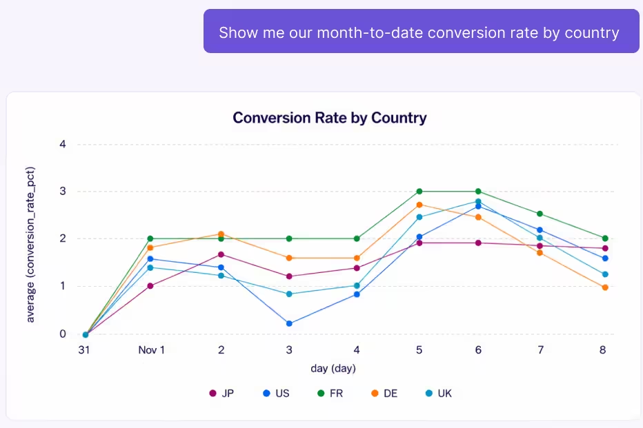
Make the evaluation replayable before making it large
Establish a small output contract
You can test the evaluation plumbing without choosing a provider or spending money on generation. Start with saved model outputs and a deterministic scorer. The example below evaluates a deliberately narrow contract: each support answer must choose the expected action and cite at least one source from the case's allowlist.
This is a replay test of captured outputs. It does not call a model, assess prose quality, verify factual support, or prove that a prompt performs well. Its purpose is to catch broken data joins, incomplete runs, and obvious contract failures before those mistakes are multiplied across a larger evaluation.
Use Python 3.9 or newer. Create a new empty directory and save these 2 lines as cases.jsonl. Each line is a separate JSON object:
Save these synthetic results as outputs.jsonl. There is one result for each case and variant in trial 0. The candidate deliberately fails the second case:
Keep a real runner's raw response separately from its parsed output. Parsing failures should remain visible as invalid results rather than being repaired by an undocumented cleanup step. Python's JSON parser and encoder provide the basic loading behavior; the product-specific validation rules belong to your harness.
Fail incomplete comparisons instead of hiding them
Save the following as score_replay.py. It requires a complete baseline/candidate pair for every expected case and trial, rejects duplicate and unknown result IDs, and reports provider errors separately from contract failures. The positional command-line argument sets the number of expected trials per case.
Run the scorer from the directory containing the 3 files:
The baseline should report a case mean pass rate of 1.0, the candidate 0.5, and the paired difference -0.5. Those are fixture results, not claims about any model. The missing-date slice reveals exactly where the candidate regressed.
Now remove one result row and rerun. The script should raise a missing-results error. Restore the row, change its status to error, and rerun: the process should exit with status 2 and report execution errors. This verifies that a broken run cannot quietly become a reassuring quality score.
Extend the harness without changing its meaning
For real evaluations, your existing application runner generates the same result envelope from each prompt revision. Replace synthetic responses with captured outputs, retain the raw provider response, and attach the run manifest. For repeated generation, emit trial IDs from 0 through the configured count minus 1. The scorer rejects missing repeats.
Add checks that match your application: output schema, allowed tool names, required fields, or an end-state assertion in a sandbox. Do not use a substring check as a factuality evaluator. A source ID can exist while the answer misrepresents the document. An action label can be correct while the explanatory text is misleading.
The script intentionally gives every case equal weight and every trial within a case equal weight. It does not produce a confidence interval, calculate traffic-weighted performance, or certify a release. Preserve that distinction when you replace it with a larger platform. A sophisticated dashboard can hide the same denominator mistakes as a short script.
The scorer also exits successfully after reporting a quality regression: it is a diagnostic, not a CI release gate. If you automate promotion, implement an explicit separate decision step that reads the results and enforces your predeclared requirements. Verify that step with a known failing fixture. Otherwise, CI may interpret “the scorer ran” as “the candidate passed.”
Calibrate judgment before trusting a quality score
Use a rubric that separates independent questions
Contract checks answer questions whose rules are explicit. Human or model grading addresses questions such as whether a response is supported, complete, and useful. Keep those scores separate so an improvement in tone cannot compensate for an incorrect refund decision.
A practical rubric for the support example asks 3 questions: does every policy claim follow from the provided evidence, does the response identify the information needed for the next step, and does it make an unsupported promise? Define pass and fail examples for each question. “Helpful: 4 out of 5” is difficult to audit when nobody can explain what distinguishes a 3 from a 4.
Use reference information rather than trusting a judge's general knowledge. Show the policy excerpt, relevant account facts, and the output being evaluated. Ask for the verdict plus a short explanation tied to evidence. Keep the verdict in a machine-readable field and retain the explanation for debugging.
Managed evaluation systems distinguish model-based and computation-based metrics. That separation is useful even in a small custom harness: choose the cheapest reliable method for each requirement, then reserve judgment for requirements that cannot be checked directly.
Test the grader against people and counterexamples
Before applying a model judge across thousands of outputs, compare its verdicts with domain reviewers on a labeled calibration set. Include clear passes, clear failures, and borderline examples. Review disagreement by failure type rather than relying only on one agreement percentage.
A grader can agree often by passing almost everything when most examples are good. Inspect whether it catches unsupported claims, unnecessary refusals, and wrong next steps. If the product's critical failure is a false promise, the grader's ability to detect that failure matters more than agreement on easy formatting cases.
Blind candidate labels when possible and vary response order in pairwise comparisons. LLM judge research documents position, verbosity, and self-enhancement biases. A longer response winning more often is not sufficient evidence that it solves the task better. Test shortened, reordered, and intentionally flawed answers to see what your own grader rewards.
Version the rubric and judge configuration. When either changes, rescore both baseline and candidate outputs. Reusing old baseline grades with a new judge creates a comparison between evaluation methods as well as prompts. A grader migration deserves its own calibration record.
Treat repetitions as reliability evidence
Run repeated trials when generation variability could change the decision. A single output tells you what happened once. Repeats show whether a case is usually handled correctly or only occasionally succeeds. They do not create new user scenarios.
Suppose you evaluate 100 distinct tickets 5 times each. You have 500 generations, but still only 100 ticket contexts. If a rare policy situation is missing, repeating common tickets will never add it. When estimating performance across cases, preserve that grouping rather than pretending all 500 observations represent independent customers.
Compare candidates on the same cases. Inspect cases that improve and cases that regress, not only the net difference. For a formal uncertainty estimate, use a method that respects the sampling and dependence structure, such as resampling independent case groups for a paired bootstrap. Keep conversations or account clusters together when they generated related cases.
Predefine the comparison that will support your decision. Trying many prompt variants and presenting only the best held-out result invites selection bias. Use the development set to narrow the field, then assess a small finalist set under a documented rule. If the result remains uncertain, name that uncertainty rather than treating a marginal ranking as a proven gain.
Consider a hypothetical paired comparison across 200 independent cases. The candidate fixes 18 baseline failures and breaks 12 baseline passes. Its net gain is 6 cases, or 3 percentage points. That aggregate can conceal a serious problem if most of the 12 regressions concern an important policy exception while the fixes involve cosmetic preferences. Retain the paired change list and review the severity and slice of each transition.
Do not describe a 3-percentage-point difference as a 3% relative improvement. If the baseline passed 80% of cases and the candidate passed 83%, the relative increase in pass rate is 3 divided by 80, or 3.75%. Neither number establishes statistical precision by itself. Report the raw counts, denominator, and metric definition before deciding which summary best communicates the change.
A model judge's confidence field is a separate quantity again. Unless you have validated its calibration, a self-reported confidence of 0.9 is not a 90% probability that its verdict is correct. Use observed agreement and error patterns on adjudicated cases to decide how much review the grader needs. Keep unresolved grader failures as unknowns that require investigation, not as automatic passes.
Scale execution without changing the measurement
Budget the whole evaluation graph
Generation count grows as cases multiplied by variants multiplied by trials. Judge calls and multi-turn interactions add to that total. A hypothetical run with 1,000 cases, 4 variants, and 3 trials already requires 12,000 generations before grading. If each generation receives 2 model-judged checks, that is another 24,000 grading operations unless you deliberately combine or sample them.
Estimate tokens, execution time, and spend before starting. Use observed input and output sizes from a small pilot rather than assuming every case costs the same. Long-context cases and agent trajectories can dominate the budget. Set a maximum run budget and decide what the runner does when it reaches it.
Use tiers. Run cheap contract checks on every change, a broader regression set before merge, and a larger finalist evaluation before release. Periodic full runs can detect gaps that a small smoke suite misses. The point is to align expensive evidence with the decision it informs, not to make every keystroke trigger the largest possible run.
Bound workers, retries, and timeouts
Start with a small concurrency limit and measure throughput, provider errors, and latency. More workers can create rate limiting that makes the run slower and changes which cases complete. Evaluation runner controls for concurrency, repetition, and timeouts illustrate the operational settings worth making explicit, whichever harness you use.
Give each request a timeout and the entire run a deadline. Retry transient failures with a bounded policy, recording every attempt. Keep transport retries separate from new model trials: a retry after a timeout may incur cost even when you never received the original output. It must not silently become another independent quality sample.
Persist completed results incrementally with stable identities. A resumed run should execute missing work and preserve existing results, not duplicate successful rows. Write a completion receipt containing expected results, observed results, execution errors, and the manifest ID. A green process exit is insufficient if the queue never scheduled half the cases.
For a run with 1,000 cases, 2 variants, and 3 trials, the receipt should account for all 6,000 expected result identities. Suppose 5,940 succeeded and 60 ended in provider errors. Completion coverage is 99%, not 100%, and the missing 1% may be concentrated in one variant. Investigate that pattern before interpreting a small quality difference. Budget exhaustion, an interrupted worker, and a refusal are different events and need different result categories.
Keep human review in the execution plan as well. Review a random sample to estimate ordinary grader error, then add a targeted sample of disagreements, novel slices, and critical failures for diagnosis. Label which sample produced which conclusion. A targeted audit can find important defects efficiently, but its error fraction does not estimate the overall error fraction without accounting for how it was selected.
Report failures by variant and slice. If a candidate times out more often on long inputs, excluding those cases can make its completed responses look unusually strong. The replay scorer blocks an aggregate quality comparison when execution errors occur; a production harness can support a richer analysis, but it should still show completion coverage and operational failures alongside quality.
Make caching, isolation, and data handling explicit
Cache keys should include everything that affects generation: prompt revision, model settings, input, retrieved context, and tool configuration. Judge caches also need the rubric and judge revision. Reusing an output after one of those changes may save money while invalidating the comparison.
Repeated trials need independent generation when the goal is to measure variability. Test-runner repeat and cache behavior is worth checking explicitly; a repeated row in a report is not proof that the provider was called again. Record whether each response was fresh, cached, or resumed.
For stateful agents, reset the sandbox between trials. A test account that already received a refund is a different starting condition from a fresh account. Separate evaluation traffic from live user actions and verify the resulting state, not just the assistant's claim that an operation succeeded.
Apply your normal data controls to stored inputs and outputs. Scrub unnecessary personal information, limit access, define retention, and use approved providers and environments. Redaction must preserve the variables that matter to the task. Removing all dates from a refund case protects less than you think if it also makes the expected answer impossible to determine.
Promote one finalist into a measurable production test
Choose an assignment unit that matches the experience
An offline finalist is a candidate for controlled exposure. It is not yet evidence of improved retention, conversion, or task completion. The difference between AI evaluations and A/B tests matters because a response that satisfies a rubric can still be slower, harder to use, or less effective for real customers.
Use a stable user, account, or conversation identifier for assignment, depending on how the experience persists. A support conversation usually should not switch prompts halfway through because a request was randomly assigned again. When coworkers share an account-level workflow, consider whether assigning individual users would mix experiences inside one organization.
Serve the chosen immutable prompt revision through the application and keep a known-good fallback. Feature flag based prompt routing provides a useful production pattern. GrowthBook's feature flags supply configurable delivery rules alongside experiment assignment; your application still invokes the model, handles its response, and enforces any action authorization.
Do not treat a flag evaluation as proof that a user received an answer. Track assignment, request execution, delivery, and downstream outcomes as separate events. That distinction lets you detect a candidate that looks good among delivered answers because many assigned requests failed before delivery.
Join exposure, delivery, and outcomes deliberately
The following is an example of an application-owned delivery event. These field names are illustrative; map them to your tracker and warehouse schema rather than sending this object to an invented GrowthBook ingestion endpoint:
Verify that the request ID connects this event to a generation attempt and that the assignment identifier connects to the outcome metric. Keep assigned failures in the primary analysis population when the question is the effect of assigning the experience. A delivered-only comparison can be a diagnostic, but delivery is itself something the treatment may change.
GrowthBook's data source configuration defines the assignment query and identifier types used for experiment analysis. Its Fact Tables and metrics let you define outcomes from your warehouse data. The critical implementation work is making the identifiers, timestamps, and observation windows line up; a dashboard cannot repair a join between incompatible IDs.
Maintain a small instrumentation audit alongside the experiment. Count assigned units by variation, missing request identifiers, generation failures, delivered answers, and outcomes that arrived after the observation window. Check whether a user can appear under multiple variations and whether identifier changes at login create duplicate subjects. These checks can reveal an implementation problem before you spend time debating the prompt.
Allow delayed outcomes to mature. A response may look successful immediately because the user stops messaging, then produce a reopened ticket the next day. Define resolution and reopening windows before launch and give recently exposed users enough time to complete them. Comparing a mature baseline window with an immature candidate window can create an apparent improvement that disappears as data arrives.
Choose a primary user outcome such as successful self-service resolution within a defined window. Add operational guardrails for errors, latency, and escalation, with definitions agreed before launch. A decrease in escalations is not automatically good if users give up instead. Track a success signal that cannot be improved merely by withholding help.
Rehearse a decision you can act on
Before broad exposure, verify baseline assignment, candidate assignment, a failed generation, a delivered response, and the fallback path in a test environment. Confirm that the warehouse receives the expected records and that outcomes join to the intended assignment unit. Check that an operator can restore the known-good revision and observe the change after your actual refresh and caching delays.
Set the run duration, minimum worthwhile effect, analysis method, and stopping rule before reading results. If you need frequent interim decisions, use an analysis method designed for that monitoring pattern. Repeatedly checking an ordinary fixed-horizon p-value and stopping at the first favorable result changes the false-positive risk.
Warehouse-based experimentation connects this production decision to the metrics your team already uses. It complements the offline harness: the harness protects task requirements and known regressions, while the experiment measures the effect of offering a particular experience to a defined population.
Start with one consequential prompt, a versioned baseline, a small trustworthy case set, and a complete run receipt. Expand the dataset when coverage is missing, add repeats when variability obscures the decision, and add workers when execution is the bottleneck. Those are different problems. Solving the one your system actually has is what makes prompt testing work at scale.
Measure your next prompt release
Use GrowthBook to assign a tested prompt candidate and measure its effect on user outcomes alongside operational guardrails.
Get Started With GrowthBook
Related Articles
T-statistic explained: What the t-value tells you about your results
An experiment report shows a t-value of 2.4. Is the product change large? Is it beneficial? Does it have a 95% chance of working? That single number cannot answer those questions.
A t-statistic compares an estimated quantity with a hypothesized value, using the estimate’s standard error as the measuring stick. It compresses the size of the observed departure and the precision of the estimate into one signed number. Understanding the two parts is more useful than memorizing a cutoff.
For experiment readers, the essential habit is to unpack the t-value before interpreting it. Establish what was subtracted, which uncertainty estimate sits underneath it, and what reference distribution applies. Then return to the effect in product units and the decision it needs to support.
Read t as a difference divided by uncertainty
Identify the numerator and its direction
The general structure is:
In an independent treatment–control comparison, the estimated quantity might be the treatment mean minus the control mean. With a null difference of zero, a positive t means the estimated treatment mean is higher. Reverse the subtraction order and the sign reverses.
“Higher” does not necessarily mean “better.” More purchases may be desirable; more errors usually are not. A negative latency difference can support an improvement, while a positive error-rate difference can indicate harm. Read the direction in the metric’s own terms before assigning a business meaning to the sign.
The hypothesized value also matters. The usual zero-difference comparison asks whether the population mean difference is zero. Testing another specified difference changes the numerator. Neither calculation independently establishes an equivalence or non-inferiority claim; those require the appropriate hypotheses, margins and decision procedure.
Distinguish standard error from standard deviation
An observation standard deviation describes spread among observed unit outcomes. A standard error describes uncertainty in an estimator, such as a sample mean or a difference between means. They can share units while answering different questions.
For an ordinary mean of independent, identically distributed observations with finite variance, the estimated standard error is the sample standard deviation divided by the square root of the sample size. The standard-error calculation therefore changes when the number of independent observations changes, even if their measured spread stays the same.
This is why dividing a mean difference by the observation standard deviation does not give the usual two-sample t-statistic. It omits how precisely the means were estimated. The distinction between standard error and standard deviation is the first denominator check to make when a t-value looks surprising.
Unit-free does not mean effect size
Both numerator and standard error have the same measurement units, which cancel in their ratio. Converting a revenue analysis from dollars to cents multiplies both by 100 and leaves t unchanged. That is a useful consistency check for a positive linear change of units.
However, t does not describe the size of the product effect independently of precision. An observed difference of one dollar can have a small or large t-value depending on the standard error. Comparing t-values across two experiments is therefore not a reliable way to rank their business impact.
The statistic measures departure from the null in estimated standard-error units. Keep the raw difference beside it so the unit-free summary does not displace the quantity the team actually needs.
The calculation also needs a usable, positive estimated standard error. A zero or undefined denominator is a reason to inspect the data and model, rather than manufacture a finite t-value or call the result certain. Software may reject such inputs; for example, the R t-test reference documents an error for effectively constant input data.
Match the denominator to the study design
Different designs estimate different uncertainty
The formula’s short form hides a substantial choice: how was the standard error calculated? Three common cases illustrate why the design must come first.
| Design | Estimated standard error | Reference degrees of freedom |
|---|---|---|
| Ordinary one-sample mean | Sample SD divided by √n | n − 1 under the classical model |
| Ordinary paired mean difference | SD of within-pair differences divided by √number of pairs | Number of independent complete pairs − 1 under the classical model |
| Independent Welch comparison | √(s² treatment / n treatment + s² control / n control) | Welch–Satterthwaite approximation using both group sizes and variances |
In the paired case, the relevant spread is the spread of differences within pairs. Substituting the two arms’ separate standard deviations discards the relationship the design uses. The paired t calculation treats the differences as its observations; the independent information comes from the pairs.
For two independent groups, Welch’s calculation does not require equal population variances. The pooled Student calculation adds that assumption and uses a different variance estimate. The Welch-versus-Student comparison helps distinguish those cases. A label reading only “t-test” can conceal the choice.
Separate a reference model from an arithmetic ratio
You can calculate a difference divided by an estimated standard error without proving that the resulting statistic has the reference distribution you intend to use. Exact classical one-sample and paired t inference relies on the corresponding independent normal-observation model; in the paired case, this concerns the differences.
Welch’s reference distribution is an approximation with estimated degrees of freedom. It is not generally exact even for unequal-variance normal populations. Non-normal outcomes can support useful large-sample mean inference under appropriate conditions, but there is no sample-size threshold that makes every heavy tail or dependence problem disappear.
If accounts are randomized, individual events from one account are not automatically independent units. A standard error that ignores the account structure may understate uncertainty. More rows in an exported file do not by themselves justify a smaller denominator or larger degrees of freedom.
Plan for more precise estimates
Explore variance-reduction methods and their tradeoffs before your next test. Match each method to the outcome you intend to estimate.
Explore Variance Reduction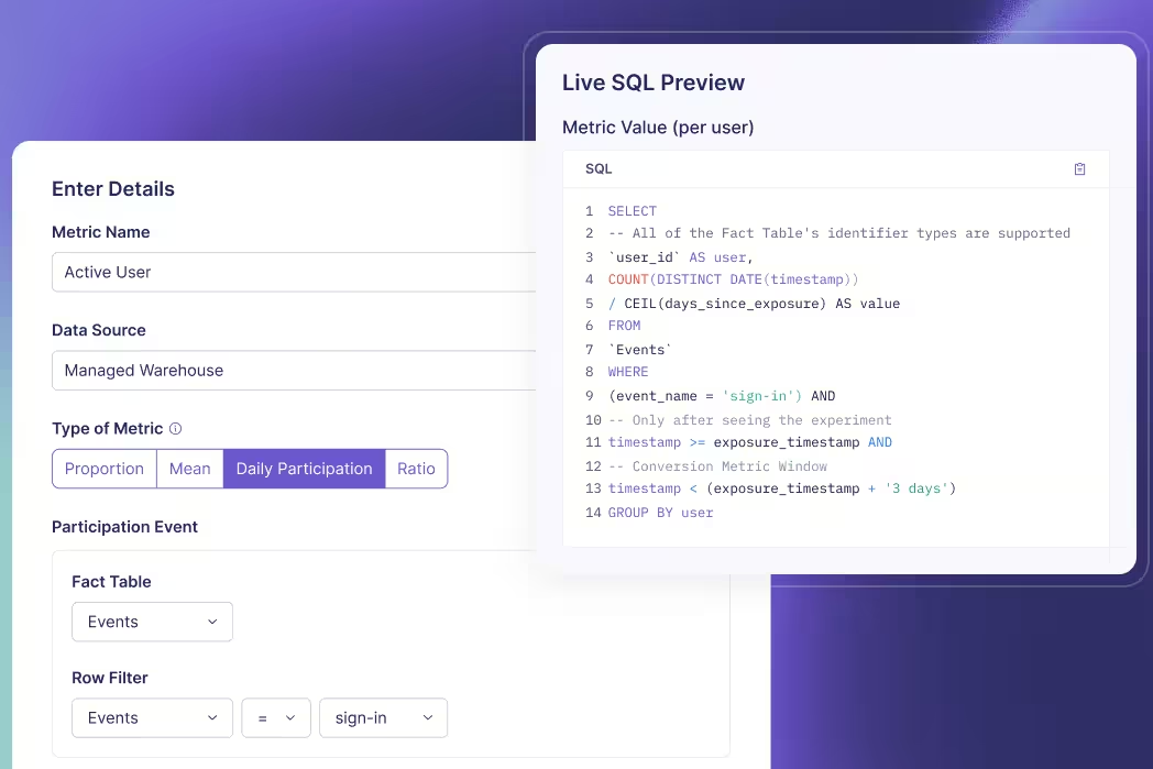
Hold the observed effect fixed and change precision
Work through an independent mean comparison
Consider a hypothetical fixed-horizon experiment with one completed revenue outcome per independent user. Control has mean revenue of $10; treatment has $11. Each arm has sample standard deviation $4 and 100 users. The target is the arithmetic mean difference, treatment minus control, and the null difference is zero.
The estimated effect is $1 per user. Using the independent unequal-variance standard error, square each group’s standard deviation, divide by its sample size, add those terms and take the square root. Here that is √(16/100 + 16/100), or about $0.5657.
Divide the $1 difference by $0.5657 to get t ≈ 1.7678. The estimated difference lies about 1.77 estimated standard errors above the zero-difference null. The sample standard deviation is still $4; the $0.5657 figure measures uncertainty in the difference between the two estimated means.
For these equal sample sizes and equal observed variances, the Welch–Satterthwaite calculation gives 198 degrees of freedom. Under the conventional Welch approximation, the two-sided p-value is approximately 0.07864 and the 95% confidence interval for the mean difference is approximately −$0.1155 to $2.1155.
Compare two hypothetical studies
Now consider a separate hypothetical study with the same group means and standard deviations, but 400 independent users per arm. The observed $1 difference has not grown. Its estimated standard error is smaller.
| Summary | 100 users per arm | 400 users per arm |
|---|---|---|
| Observed mean difference | $1 | $1 |
| Sample SD in each arm | $4 | $4 |
| Estimated SE of the difference | $0.5657 | $0.2828 |
| t-statistic | 1.7678 | 3.5355 |
| Welch reference df | 198 | 798 |
| Conventional two-sided p-value | 0.07864 | 0.0004304 |
| Conventional 95% CI for the difference | [−$0.1155, $2.1155] | [$0.4448, $1.5552] |
Quadrupling each group’s sample size halves the estimated standard error when these observed standard deviations stay fixed. It doubles t for the same observed effect. The larger statistic reflects greater estimated precision here, not a larger observed revenue gain.
These are teaching summaries for separate studies. They are not an instruction to keep extending one experiment until significance appears. In a real extension, means and variances can change, and the stopping rule affects how the inference should be calibrated. An observed t-value also does not directly tell you the power of a future study.
Translate t using the appropriate reference distribution
Degrees of freedom and tails determine the threshold
A t-value needs a reference distribution before you can obtain a p-value or critical value. The Student t family includes a degrees-of-freedom parameter; smaller values generally give heavier tails. The same absolute statistic can therefore produce different tail probabilities at different df.
For a prespecified two-sided 5% test, the relevant critical value is the 97.5th percentile of the reference t distribution. It approaches about 1.96 as df becomes large, but 1.96 is not a universal t cutoff. Nor does every test use n − 1. Degrees of freedom depend on the calculation and may be fractional for Welch.
A one-sided alternative uses a specified tail and a different critical value. A negative statistic is not evidence in favor of an upper-tail alternative simply because its absolute value is large. Choose the direction before seeing outcomes; taking whichever tail looks favorable changes the decision rule.
A p-value conditions on the null model
For a conventional two-sided t-test, the p-value is the probability, under the null model and assumptions, of a statistic at least as extreme in either direction as the observed t. It is not the probability that the null is true, that chance caused the result, or that a future experiment will succeed.
The ASA’s p-value principles also distinguish statistical significance from effect magnitude and practical importance. A threshold crossing does not determine whether the expected benefit pays for the change. If you need the broader conditional-probability interpretation, the t-test p-value guide develops it separately.
Read the interval in the original units
The corresponding conventional interval is the estimated difference plus or minus the relevant critical t-value times its estimated standard error. For the same two-sided procedure at 5%, a 95% interval excluding zero agrees with rejecting a zero-difference null. That agreement requires compatible test, interval and adjustment settings.
Confidence describes the repeated-use coverage of the method under its assumptions. It does not assign a 95% posterior probability to the fixed true effect lying inside the particular computed interval. The confidence-interval construction makes the relationship between standard error, critical value and width explicit.
In the first study, the interval includes a small loss and a substantial gain. In the second, it excludes zero but still spans different levels of business value. A minimum worthwhile effect helps interpret that range. Neither a large p-value nor an interval containing zero proves equality; equivalence requires an analysis designed for that claim.
Audit the inputs before acting on a t-value
Trace an unexpected statistic to its components
Start with the estimated effect and null value. Confirm the subtraction order, currency or time units, eligible population and observation window. A swapped group order explains a sign change; it does not explain a change in a correctly calculated two-sided p-value.
Then inspect the denominator. Check group sizes and sample variances at the actual independent unit. Look for duplicated joins, repeated events counted as independent observations, incomplete follow-up and treatment-dependent missingness. The arithmetic can be internally consistent while the data fail to represent the intended experiment.
Inspect the analysis settings too. A ratio metric, regression adjustment or variance-reduction method can have a standard error different from the simple independent-mean formula above. Do not attempt to reproduce a dashboard by substituting top-line traffic counts into the wrong calculation. GrowthBook’s statistical effect calculations describe its estimators and frequentist reference methods, including distinct metric types.
Keep the decision rule attached to the evidence
The worked examples use conventional fixed-horizon inference. Repeatedly inspecting that calculation and stopping at a favorable threshold changes its false-positive behavior. A planned sequential analysis is a different inferential procedure; GrowthBook documents an asymptotic confidence-sequence approach with its own settings. It does not repair incorrect units or missing outcomes.
Likewise, selecting the largest t among many metrics, variants or segments creates a testing problem beyond a single comparison. Preserve the planned comparisons and applicable corrections rather than treating the most impressive number as an isolated result.
A useful readout names the estimated effect, interval, test, df, direction and sample sizes, followed by the measurement checks and decision threshold. The team can then assess what the evidence supports and whether that effect is worth shipping. Use the t-value to understand precision relative to the null; keep the launch decision grounded in effects on users and the business.
Review the result in context
Open the official experiment-analysis workflow to inspect saved results, health checks and analysis settings with configured API access. It can refresh a result snapshot when needed; stopping or rollout is separate.
View the Analysis Workflow
A published Strapi document is content. An A/B test also needs an assignment, a delivered experience, and an outcome you can attribute.
The integration becomes unreliable when those pieces disagree. An older example may read data.attributes, while your Strapi 5 endpoint returns flat fields. A numeric database ID may be mistaken for a document ID. An internal service call may return a draft even though a similar REST request defaults to published content.
This guide builds an explicit Strapi 5 content test using a small server-rendered Node application and GrowthBook. It validates the complete published content pair before enrolling a visitor, preserves a stable browser identifier, and records an exposure only after browser execution reaches the selected page.
The code also fingerprints the reviewed strings so a later edit can be rejected before assignment. The local event collector demonstrates the measurement boundary; a real experiment still needs your existing signup flow, durable analytics delivery and verified warehouse joins.
Define the Strapi 5 delivery contract
Pick a content model you can inspect
The existing GrowthBook Strapi integration guide demonstrates Dynamic Zone components selected through a frontend SDK. The reference here uses two ordinary string fields and server-side evaluation. It does not require a separately installed Strapi experimentation plugin or depend on an unverified plugin compatibility claim.
Start with a hypothesis about a meaningful outcome: an outcome-focused headline will increase completed trial signups per eligible offer-page visitor. Keep the offer and signup destination consistent if headline copy is the intervention. If the change includes a larger component package, describe that package as the treatment.
A plain-text pair makes the first integration easier to inspect. You can verify the exact response, render the selected value safely, and compare the approved strings. When extending the model to components or Dynamic Zones, validate their full structure and use a reviewed variation mapping. Reordering an array must not silently redefine which experience belongs to control.
For example, an editorial interface might place an alternative card first because it is easier to find, while the frontend still interprets index zero as control. The content can remain valid JSON and render perfectly while the experiment labels have effectively switched. Use explicit variation keys or a constrained, reviewed ordering contract when extending the simple pair. Check the rendered package against the experiment mapping, not just that every component has a title.
Use the document API that your code actually calls
Strapi 5 REST responses expose normal content fields directly under data. The document endpoint uses documentId; the numeric id in a response is not the identifier this guide puts in the URL. Some plugin endpoints have different response conventions, so this contract applies to an ordinary generated collection endpoint.
The production request explicitly sets REST status to published. This is also the REST default when Draft & Publish is enabled. The internal Document Service API defaults differently, to draft. Do not transfer that internal default—or an older v4 parameter—into this REST implementation.
Keep locale explicit as well. The requested document and locale together identify the content version being delivered. This guide checks the returned locale instead of borrowing another CMS's fallback behavior or assuming a valid document ID means every translation exists.
The document concept groups localized and draft/published variations around a document identifier. That does not make the document identifier an immutable snapshot of the text. Keep source identity, publication state and approved content as separate fields in the experiment record. Changing one is a deployment decision even when the others remain familiar.
Define assignment and measurement before launch
Use one stable assignment unit. The example creates an anonymous first-party browser ID; account-level interactions may require account assignment instead. Plan the anonymous-to-authenticated transition so signup measurement does not lose the identifier or enroll one person under several unrelated IDs.
Choose a primary business outcome, a small diagnostic funnel and relevant guardrails. A headline can increase button clicks without increasing completed or qualified signups. Estimate eligible traffic and the effect that would change your decision before starting a test that cannot resolve the question in a useful period.
Separate content ownership from experiment operation. An editor approves the published pair, an engineer owns delivery and fallback behavior, and the analytics owner verifies exposure and outcome data. Name who can change the tested content and how a change starts a new reviewed comparison.
Model, publish and inspect the content pair
Create a localized collection in development
Use an existing Strapi 5 test application with Draft & Publish enabled for the collection. Configure internationalization and the intended locale if the content is localized. The Content-type Builder belongs to the development workflow; deploy schema changes through your normal application process.
Create a collection named Experiment page with singular API ID experiment-page and plural API ID experiment-pages. A minimal schema at src/api/experiment-page/content-types/experiment-page/schema.json is:
For an existing model, merge the relevant changes rather than replacing its other fields. Restart or rebuild according to your development workflow, create a document, enter both approved headlines and publish the intended locale. Copy its actual documentId from the API response or your document inspection workflow.
Review model changes and content changes through their appropriate paths. Adding a field affects application schema and deployment; editing a headline changes a content entry. Give the editor clear field descriptions so control means the approved baseline and variant means the approved experimental alternative. A required field helps authoring, but the renderer still validates the actual response from the deployed endpoint.
With internationalized content, inspect the specific localized pair that will be eligible for the experiment. Translating control but leaving treatment in an unintended language changes more than the hypothesis describes. Keep locale targeting and content approval aligned, and decide in advance whether results across languages belong to one planned analysis or separate comparisons.
Because both alternatives are plain strings, this request needs no relation population. Components, relations and media require an explicit population strategy when added later; populate=* is not a substitute for defining the treatment's dependencies and permissions.
Use a read token on the rendering server
Create a scoped Content API token for the renderer. A read-only token supports find and findOne; a Custom token can narrow the relevant endpoint access. Keep it on the application server. You do not need to expose an admin token or broadly enable public-role access for this authenticated server request.
Read-only describes allowed operations, not a universal guarantee that a caller can never request drafts. Fix production status and locale in trusted code. Keep editor preview routes and any draft-capable configuration separate from live enrollment and analytics.
When extending the endpoint with a language switcher, select from an approved locale set rather than forwarding every browser query parameter to Strapi. A request parameter named status should not turn the production renderer into a draft-content proxy. Keep the collection path and publication choice fixed, and validate the returned document and locale even after constructing a valid request.
Check permissions on the actual route you use. A working admin interface does not prove the rendering token can read the generated Content API endpoint. Conversely, an access problem is not a reason to grant broad public access to the entire model. Confirm the token's scope and the endpoint response independently of experiment assignment.
Create a reference Node project, or integrate the files into your existing application. Use a modern Node runtime compatible with the locked dependencies, such as Node 22 or later:
Add server configuration. STRAPI_ORIGIN is the CMS origin, including a port when needed, without /admin or /api appended:
Use the appropriate HTTPS origin outside your local development setup. Store credentials through your deployment's configuration mechanism, not in public HTML or query parameters.
Validate the published response and reviewed fingerprint
The following reader fetches one document by documentId, with explicit locale selection. It rejects a missing, draft, wrong-locale or malformed pair before the SDK can assign anyone:
Leave the optional expected hash blank for the first read-only inspection, with Strapi running and the document published. Run:
Confirm the actual approved pair, source origin, document and locale. Set STRAPI_EXPECTED_SHA256 to the returned digest before enrollment. The SHA-256 calculation fingerprints those exact strings and source dimensions. It does not retrieve an older Strapi version or grant access to anything.
documentId, updatedAt and publishedAt are useful context, but they do not freeze a treatment. The fingerprint rejects changes to the reviewed pair before assignment. Identical strings can retain the same digest after republication; publication metadata is recorded separately. Extend the fingerprint when additional content becomes part of the treatment.
Treat updating the expected digest as a review step. First inspect the new delivered pair, confirm why it changed, and decide whether the current experiment can continue under a documented phase or needs a new experiment. Copying the latest digest merely to clear an unavailable response defeats the check. Preserve the approved strings alongside the digest so a reviewer can understand the change without reconstructing it from a hash.
The digest covers the two headline strings and source dimensions in this implementation. It does not cover an unrelated image, price, signup destination or application deployment. If those become part of the intervention, extend the reviewed package and its validation. A useful content contract is explicit about both its coverage and the changes that require another review.
Review the experiment before launch
Open the experiment-design workflow to turn your content hypothesis, assignment unit, and metrics into a reviewable specification. Configure API access as directed and review the plan before launch.
Open Experiment Design InstructionsRender the assigned page with request-local context
Link the content values to an experiment
Create a string feature strapi-offer-copy, defaulting to control. Link an experiment with tracking key strapi-offer-copy-v1, mapping the two string values to the intended variations. Set hash attribute id, the correct SDK environment, targeting and goals in the experiment configuration.
The content value chooses a string from the pair. The experiment and variation identifiers describe the assignment for analysis. Preserve experiment.key and result.key; do not substitute the headline or assume a variation key must equal the content value.
The GrowthBook Node SDK can share feature payload data while keeping each visitor's context in a scoped instance. The server initializes through the request path and checks success, using the SDK's caching and refresh policy rather than retaining one startup promise forever. Test stopping and refreshing on warm instances; a shared cache is not an instant global update guarantee.
Keep the browser identity stable and the output safe
Create the server below. The existing /signup application flow is a prerequisite: implement or replace that link before measuring completed signups. The collector is a local diagnostic endpoint until connected to durable analytics.
The cookie parser can produce non-string values, so identity is validated before assignment. Express cookie maxAge uses milliseconds. The redirect establishes the cookie before the offer request; its one-attempt marker avoids looping when persistence fails. Adapt identity and consent behavior to the application's existing policy.
The headline is escaped as HTML text. The JSON data element separately escapes less-than signs so a closing-script sequence cannot terminate it. These are different output contexts. Do not use this plain-string renderer as a general HTML or Rich Text renderer.
Keep failure behavior visible
A missing document, wrong locale, draft payload or changed fingerprint fails before enrollment. A failed feature-payload initialization can retain valid control content outside enrollment. Unexpected raw assignment values are logged and do not become misleading control-view events.
Fetching both alternatives in one validated payload makes this eligibility check independent of the assigned arm. A different architecture that first assigns treatment and then fetches only its content has another failure problem: a missing treatment resource can selectively remove treatment visitors from observed exposures. If larger packages require that architecture, preserve assignment and delivery failures explicitly and design the analysis population before launch. Do not infer that a missing view means the visitor never belonged to the comparison.
Preserve diagnostics and investigate the affected interval. Filtering failed treatment deliveries from analysis can select the comparison population after assignment. A safe display fallback does not make a broken experiment trustworthy; repair or halt it when delivery or configuration is unreliable.
The personalized response uses private, no-store. Shared caching of the complete validated pair is a separate choice from caching a visitor's selected HTML. Verify the actual reverse proxy and CDN behavior rather than assuming a response header alone describes every cache in the deployment.
When adding a shared content cache, include the CMS instance, document, locale, publication selection and reviewed fingerprint in the appropriate cache design. A cached English pair should not satisfy a request for a different locale, and a previously approved pair should not conceal a broken publication process indefinitely. Test invalidation and recovery using the same deployment configuration as the experiment.
The server selects one headline before producing HTML, so the browser does not need to rewrite that headline to implement this treatment. Measure the server response path under realistic load nonetheless: content fetching, payload initialization and application work still consume time. Keep loading and error guardrails appropriate to the page rather than promising that server-side evaluation has no performance cost.
Connect browser exposure to the outcome
Record a defined display boundary
The callback during evaluation queues assignments; it is not proof that HTML reached a browser. Use the deferred-tracking pattern to carry compact metadata into a client script that runs after parsing the page:
This boundary establishes that browser execution reached the rendered page. It does not prove viewport visibility or reading. Use a symmetric visibility condition if that is the intended exposure definition. A successful beacon queue operation also does not prove network acceptance or durable ingestion.
The data-element marker prevents duplicate execution within one document. Reloads can produce additional displays, and collector retries need their own event-ID policy. Define whether analysis uses first exposure or another consistent rule, then make the assignment query match that definition.
Replace local logging with verified ingestion
The diagnostic collector reads identity from the HttpOnly cookie, validates the event/source fields and discards unexpected fields. It still receives browser-supplied observations. Do not use that metadata as an authorization or billing decision, and do not treat a console row as a warehouse record.
Connect your supported analytics ingestion with appropriate validation, origin controls, delivery monitoring, retries and deduplication. Apply consent and tracker-readiness behavior consistently across both arms. Compare assignments, browser events, accepted requests and warehouse rows when investigating loss; those counts represent different boundaries.
Configure the GrowthBook data source to read experiment key, variation ID, timestamp and assignment unit from the actual stored schema. Preserve the document/locale/hash provenance in the event or a linked experiment record so the content behind a result remains identifiable.
Validate that mapping with one controlled event before increasing traffic. Compare the browser request, accepted collector fields and resulting warehouse row. Field names can change through an analytics transformation, timestamps may be stored in different zones, and a custom identifier can be dropped by a tag or export. Finding the row and joining its outcome is stronger evidence than seeing a successful HTTP response from the local collector.
Join the business outcome to the same identifier
Define completed signup or another chosen outcome with Fact Tables and metrics. Verify that it joins to the browser assignment identifier or a tested authenticated-identity mapping. A signup on another origin does not automatically carry this cookie.
Inspect an actual controlled exposure and outcome together, including timestamps, duplicate handling and follow-up window. Recent visitors may not yet have had enough time to complete the outcome. Keep diagnostic clicks and qualified conversions separate so faster but less useful signals do not replace the intended decision.
Verify publication and maintain a clean test
Check HTTP behavior before interpreting results
With the reviewed hash configured, run the application and establish a local cookie jar:
Expect a fixed redirect and consistent selected content for the same identifier while configuration remains stable. These requests inspect server HTML; they do not execute the browser exposure script. Use a real browser to inspect the beacon and collector, then verify the actual analytics and warehouse path separately.
Exercise both arms with controlled identities. A forced value can prove a rendering branch, but it does not prove ordinary randomized enrollment. Keep preview, forced and employee QA traffic outside production analysis.
Persistence is also narrower than sticky assignment across arbitrary configuration changes. The same browser ID can be used consistently while a changed experiment key, rule or allocation alters the experience. Freeze the intended configuration during the comparison, record deliberate changes, and use the platform's supported bucketing behavior when your requirements extend beyond a stable identifier.
Test the modern contract and its failure cases
| Test condition | Expected behavior | What to investigate |
|---|---|---|
| v4-style nested response | Reject missing flat fields | Migration compatibility and parser version |
| Numeric row ID used as document ID | No successful content display | Actual documentId and generated endpoint |
| Draft or wrong-locale payload | Reject before assignment | Status, localization and preview configuration |
| Reviewed string changes | Hash mismatch before enrollment | Publication approval and treatment version |
| SDK, cookie or event failure | Explicit baseline/unavailable/diagnostic path | Identity continuity and delivery loss |
Also test HTML-significant characters and a closing-script sequence in approved QA content. They should remain text, and the data element should remain intact. Repeat cache and identity checks on the actual deployment: local success does not establish proxy behavior, public rendering or warehouse attribution.
Include a schema deployment in the regression check when field names or content structure change. A correct new schema in development can coexist with older published documents or a renderer expecting the previous shape. Verify the deployed model, the delivered payload and the rendering contract together. Keep a clear unavailable/diagnostic result for incompatible content rather than disguising it as a valid control observation.
Close the loop with an owned content decision
Before interpreting lift, investigate allocation anomalies, missing data and variation-specific failures. Agree on duration, outcome maturity, meaningful effect and a decision framework before seeing the result. An imprecise estimate can leave the content choice unresolved, and nonsignificance does not prove equivalence.
When the test ends, stop enrollment, verify payload refresh in deployed instances and publish the chosen headline as ordinary content. Preserve the approved pair, source document/locale, fingerprint and metric definition with the learning. Remove retired assignment and tracking branches through review so future tests begin with a clear owner and a clean content contract.
Coordinate the content promotion with the fingerprint gate. Turning the winning headline into the new control changes the reviewed pair, so approve that resulting baseline and its new digest deliberately. Test the publication/configuration sequence in staging; do not clear a mismatch by copying a new hash without checking what it represents. The final baseline should work independently of the retired experiment rule and its exposure code.
Run a clear content comparison
Connect published Strapi content to consistent assignments and the business outcomes your team already measures. Start with a small test and verify the complete delivery and measurement path.
Get Started With GrowthBook
Your randomizer can work correctly while the final experiment comparison becomes unreliable. People can enter different reporting paths, lose their identifiers, or disappear from outcome collection after assignment. The result still looks like an A/B test, but the rows left in the analysis may no longer support the question you meant to answer.
Random assignment is a powerful protection against selection into treatment. It does not guarantee representative recruitment, complete follow-up, or valid post-treatment filters. Understanding that boundary helps you distinguish an allocation problem from a problem observing the people you allocated.
The most consequential question is often what randomization lets you learn when some outcomes remain unknown. A larger sample or a more sophisticated statistical engine cannot supply those missing facts without additional evidence or assumptions.
Understand the protection randomization provides
Assignment should not depend on potential outcomes
Selection bias concerns systematic distortions introduced by how observations enter or remain in the comparison relevant to your question. The selection-bias definition emphasizes the relationship between the studied group and the population of interest. Terminology varies across fields, so name the actual selection process rather than assuming the label explains it.
With a common assignment probability, proper random assignment makes treatment allocation independent of the units’ potential outcomes. When assignment probabilities vary across prespecified strata, that independence is conditional on those strata. Product teams do not have to identify every motivation, prior preference, or unmeasured characteristic before assigning users. The allocation mechanism avoids deliberately routing more promising users into treatment and less promising users into control.
This protection concerns the units eligible for that randomization. It also relies on the implemented experiment matching the design: the assigned treatment must be well defined, identity must support the assignment, outcomes must be measured appropriately, and interference between units must be addressed where relevant.
Balance is an expectation, not a perfect copy
Randomization does not create two identical lists of people. A finite experiment can have chance differences in baseline behavior even when the mechanism is sound. The methodological basis of randomized comparisons is comparability on average under the design, rather than exact equality of every measured or unmeasured characteristic in every sample.
Investigate evidence of implementation failure, but do not repeatedly rerun allocation until the observed outcome looks attractive. Prespecified blocking or stratification can be legitimate design choices; changing allocation in response to favorable results is a different procedure.
Randomization also does not mean the observed difference equals the true effect exactly. Sampling or randomization uncertainty remains even with complete measurement. A confidence interval addresses uncertainty under its assumptions; it does not certify that recruitment, joins, filters, or outcome observation were valid.
There is another limit to what is observed. Each unit receives one assigned experience, so you do not observe that same unit’s outcome under the alternative at the same time. Randomization supports an aggregate comparison under the design; it does not reveal an individual causal effect for every user. Keeping this distinction clear prevents a clean experiment average from becoming an unsupported claim that every customer benefits.
Name the treatment effect you want to estimate. The effect of offering an experience and the effect among people who actually use it are different questions. Random allocation directly supports the first comparison under its assumptions; a user’s decision to adopt is not another random allocation.
Define the population and unit the design covers
Random assignment is different from random sampling
Assignment decides which experience an enrolled unit receives. Sampling concerns which units enter the study from a population. Randomizing a volunteer beta group can support a comparison inside that beta, while leaving a separate question about whether its result applies to customers who did not volunteer.
A narrow study is not automatically a failed study. An Android-only feature may appropriately be tested among eligible Android users. A launch claim about all platforms needs additional support. State the population, setting, and time period in the decision before debating whether the sample is representative enough.
The broader selection-versus-sampling comparison explains these categories and post-treatment subgroup examples. For an experiment review, the immediate task is to identify which population your assignment actually covers and whether the final analysis preserves it.
Choose identity and eligibility before treatment changes them
Eligibility should describe who can meaningfully receive the tested experience, using information that the treatment cannot already have changed. A supported device or an account state measured at entry can define a relevant population. Successfully using the new experience is usually an outcome, not an equivalent entry criterion.
Choose the randomization unit to match the intervention. Assigning individual employees to different collaboration settings may create interference when they work together. Assigning accounts can address some shared-experience requirements, but changes the number of independent units and the analysis needed. Randomization-unit design guidance makes identity stability and network effects part of the experiment design, not merely SDK configuration.
In implementation, preserve the assigned unit and variation through the outcome join. A device identifier that disappears after login can create missing outcomes rather than genuine non-conversions. A changing identity can also expose one person to multiple variations. Record the identity and timing assumptions with the experiment configuration, then verify the delivered data follows them.
Define the denominator first
Use the KPI playbook to distinguish binary, continuous, and ratio metrics, and connect each measurement to the experiment decision it is meant to support.
Read the KPI PlaybookMissing outcomes can defeat an apparently favorable result
Complete-case rates describe the people still observed
Suppose a hypothetical experiment assigns 100 units to each arm. The binary outcome window has ended for everyone, but a collection problem leaves some outcomes unknown. There are 18 known successes in each arm:
| Outcome availability | Control | Treatment |
|---|---|---|
| Assigned units | 100 | 100 |
| Units with observed binary outcomes | 90 | 60 |
| Known successes among observed outcomes | 18 | 18 |
| Units with unknown outcomes | 10 | 40 |
| Success rate among observed outcomes | 20% | 30% |
The complete-case comparison is 18/90 versus 18/60, an observed difference of +10 percentage points. It compares the units whose outcomes were available. It does not establish the success-rate difference for all 100 assigned units in each arm.
The larger missing fraction in treatment is a warning about observation. It is not proof of a particular direction or magnitude of bias. Equal missing fractions would not settle the issue either: equally many missing users could have different outcomes or different reasons for being unobserved.
Missingness does not inevitably create bias in every analysis. Purely random loss can mainly reduce precision; other missingness processes can select people with systematically different outcomes. The missing-value count alone does not identify which process occurred. Record the reasons for loss and what was known about affected units before treatment, rather than treating an arbitrary percentage threshold as a universal certificate of validity.
Intention-to-treat analysis with missing outcomes requires a defensible approach to those unknown outcomes. Keeping everyone’s original assignment preserves the target comparison, but the words “intention to treat” do not recover information that was never observed. Automatically assigning every missing value zero imposes an outcome assumption.
Ask what the unknown values could change
Because the example’s outcome is binary, we can calculate simple logical completion ranges. If none of control’s ten unknown outcomes were successes, its full-cohort sample rate would be 18%. If all ten were successes, it would be 28%.
Treatment has forty unknown outcomes, so its corresponding range is 18% to 58%. Across possible completions of these missing entries, the all-assigned sample rate difference could run from −10 percentage points to +40 points.
These are logical missing-outcome completion bounds, not a confidence interval and not exact bounds on a population causal effect. They hold the observed entries fixed and vary the unknown binary values. Even if every missing outcome were recovered, inference about an underlying effect would retain uncertainty from the experiment’s design.
The exercise reveals how little the complete-case +10-point result establishes without assumptions about observation. Filling all missing values with zero happens to produce 18% in both arms here. That zero difference is one completion, not a demonstrated absence of an effect.
Attrition analysis can use sensitivity checks to make missing-data assumptions visible. A useful next step is to recover outcomes from reliable records, investigate why collection failed, and assess conclusions under plausible alternatives. The most favorable completion is not a substitute for that investigation.
Preserve the comparison after assignment
Different exclusions require different repairs
Distinguish incomplete observation from a known zero. An account that was fully observed and did not purchase can legitimately contribute zero to a purchase metric. An account that no longer joins to the purchase system has an unknown outcome unless other evidence establishes what happened.
Telemetry-loss research shows why lost records can affect power and bias comparisons. Increasing traffic through the same broken collection path need not fix the problem. It may narrow the reported interval around a distorted complete-case comparison.
Inspect the metric and Fact Table definitions, including identifiers, join types, filters, timestamp alignment, and outcome availability. A left join followed by a filter on an outcome-table field can silently become an exclusion rule. A metric name does not reveal which people survived that rule.
Post-treatment filtering is another mechanism. Restricting analysis to purchasers or successful feature users can select different people in each arm when treatment changes those behaviors. Identical SQL applied to both arms does not make selected membership independent of treatment. Use such a view for a clearly limited descriptive purpose or an appropriate causal analysis; do not assume it inherits the original randomized comparison.
Triggering needs a causal and implementation argument
Analyzing a relevant triggered population can be defensible when the trigger identifies comparable eligibility across assignments. The criterion is not simply whether logging happens before or after the assignment timestamp. Ask whether the tested treatment can affect who satisfies the condition or whether that condition is recorded.
GrowthBook’s activation-metric settings explicitly warn that activation should be independent of assignment. Where a feature exists only in treatment, a carefully designed counterfactual logging approach can record who would have encountered it in control. That requires equivalent logic and validation, not just a treatment-only click event with a new name.
Passing a sample ratio mismatch check is useful evidence about allocation counts, not a guarantee that every inclusion rule is valid. Selection can change the composition of two equally sized groups. Review reasons for missingness and baseline characteristics alongside counts, rather than forcing arm sizes to match by discarding extra observations.
No statistical repair is universal. Weighting and imputation require assumptions and relevant observed information. A group absent from the data cannot be studied merely by assigning it a larger weight. A missingness mechanism related to unobserved outcomes cannot be declared harmless because a model returned a precise estimate.
For example, an imputation model may assume observed baseline information is sufficient to account for who has missing outcomes. That assumption needs a substantive argument; the unobserved values themselves cannot be inspected to verify it. Compare plausible departures from the assumption and report whether the practical decision survives. Do not choose the missing-data model because it produces the preferred launch recommendation.
Report the evidence randomization actually preserved
Track assignment separately from outcome observation
Maintain counts for eligible units, assigned units, recorded exposures, observed outcomes, and the final analysis population. Explain losses between stages by arm and by relevant baseline groups. The ledger should distinguish a known outcome from unavailable measurement, and an original exclusion from a later analytic restriction.
The data-quality requirements for online experiments include completeness, consistent assignment records, reliable joins, and timing. An allocation check alone covers only part of that path. A clean A/A test can reveal existing problems but cannot prove a future treatment will leave exposure and outcome collection unchanged.
Preserve the query or metric revision behind the result. If the team repairs a join or recovers delayed records, state whether the correction reconstructs the intended original population. If it does not, explain the resulting scope and whether a new run is needed. Avoid relabeling a selected survivor cohort as the original experiment.
Design outcome observation before increasing exposure. For an important transaction metric, a reliable backend record may allow recovery when a client event fails, provided identity and timing still join correctly. Verify that the recovery method is available in both arms and measures the intended outcome. A second event stream is useful evidence only when its own coverage and meaning are understood.
Make missing-data assumptions part of the launch decision
Alongside the experiment results, report outcome availability and the assumptions used for missing values. Transparent randomized-trial reporting treats participant flow, exclusions, and missing-data handling as information needed to judge a result. The same statistical discipline is useful for product experimentation when the participants are accounts rather than clinical-trial patients.
For the hypothetical experiment, the immediate conclusion is that the favorable complete-case result does not identify the all-assigned sample comparison without more information. The next action is to investigate observation, recover outcomes where possible, and evaluate the remaining uncertainty. It is not to declare a winner from 20% versus 30%, or a tie from zero-filled missing outcomes.
Randomization gives you a defensible starting contrast. Preserving it requires that the data and analysis continue to describe the units and outcomes the decision concerns. Before launching from a randomized result, be able to explain not only how people received a variation, but also whose outcomes are known, whose are missing, and what your conclusion assumes about the difference.
Inspect the metric definition
Open the read-only metric search workflow to find a fact metric and inspect its aggregation, filters, identifiers, and associated fact table. Running the workflow requires configured GrowthBook API access; the instructions do not execute an audit when opened.
View the Metric Search WorkflowReady to ship faster?
No credit card required. Start with feature flags, experimentation, and product analytics—free.