Should you cap outliers? Winsorization in A/B testing

What is winsorization in A/B testing?

Winsorization replaces every value above a percentile of an A/B test metric, such as the 99th percentile of user revenue, with that percentile. It’s one way to cap outliers. The other is to set the cap at a fixed value. Capping makes revenue metrics much less noisy and experiments faster. This post shows what you gain, what you risk, and when the trade is worth it.

Why everyone tells you to cap outliers

Everybody tells you to cap outliers in long-tailed metrics to gain sensitivity. Your experimentation platform has a setting for it, and every guide to variance reduction has it near the top. A key advantage is how simple it is to apply. Set a percentile, and the customers above it get their value replaced by the threshold value before the analysis runs.

If you've felt uneasy about it, you're just like me. The customers above the threshold aren't measurement errors.¹ They're your best customers, and a cap decides in advance that whatever the treatment adds above the threshold doesn't count. The variance argument is compelling, but nobody talks about what it does to your estimand, i.e. the quantity you're actually estimating.

This piece is about what made me stop worrying about capping and why I now believe it's what you want to do in most experiments. I simulate experiments with treatment effects that spread across customers differently to show what capping does to variance, point estimates, and statistical power in different situations.

The short version is that if you're deciding whether to ship a feature, you want to cap the top 1% or so, unless you expect your biggest buyers to respond much more strongly than the rest. If you need the point estimate itself, for a forecast or a business case, it's a trade-off between the bias the cap adds and the noise it removes.

Who is affected determines the impact of capping

The business setting

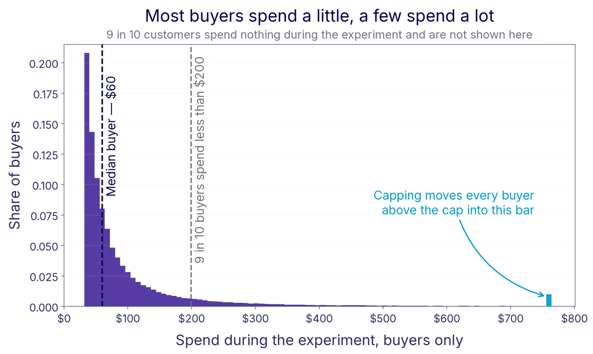
Assume an experiment with three hundred thousand customers, where one in ten buys something during the test. Spending among buyers starts around $32, the way a minimum order value works, has a median of $60, and a long tail: the 99th percentile of buyers is at $756, and the top 1% of buyers account for about 13% of all revenue. I also vary the parameters steering this distribution, so the findings can be checked against businesses with more or less concentrated revenue than this one.

In this setup I simulate the same experiment many times over, each time with a new sample of customers, a fresh 50/50 random assignment, and a treatment effect that will take different shapes. I then estimate treatment effects on revenue per customer two ways. Raw, with the values as they are, and capped at the 99th percentile of buyers. Note that here, the 99th percentile is among the buyers, i.e. ignoring the 90% of customers who buy nothing. With 10% buyers, this corresponds to the 99.9th percentile of the full sample.

Power is simply how often each version gets an estimate that's significantly different from zero. The full setup is in the appendix, and the capping explorer lets you run the same simulation with numbers that look more like your own.

Additive vs proportional effects

A treatment doesn't necessarily affect every customer the same way. What a cap costs depends on which customers are affected, so I simulate two different ways that the same 5% revenue effect can be distributed.

Additive effect. Every buyer spends exactly the same additional amount, $5 in my simulation.

Proportional effect. Every buyer increases spend by the same percentage, so the biggest customers add the most money in absolute terms.

Both are sized to give the same average treatment effect, i.e. the same increase in average revenue per customer, so the only difference between them is which customers the money comes from. In both, the treatment changes how much buyers spend, not whether they buy.

Real features rarely do exactly either. A common example is a feature that gets some customers to buy who otherwise wouldn't have, while everyone else buys what they would anyway. Those extra purchases are mostly well below the cap, so capping treats that feature almost exactly like the additive effect. The results are almost identical, so think of the additive effect as "similar for those affected" rather than "exactly the same for everyone". The proportional effect stands in for effects that grow with spend.

Now how does capping change your results under these different effect types?

How much precision does capping buy?

Capping does what it promises. In this setting the standard error of the estimate shrinks by about a third, roughly equivalent to doubling your sample size. The reduction is the same for both effect types, because the cap removes the variance coming from the tail, regardless of what the treatment did.

How much you gain in precision depends on how concentrated your revenue (or any metric value) is in the tail, and you can look up where you are (approximately) with one query: what share of your revenue comes from your top 1% of buyers? Our example setting is the middle row below.

Capping the top 1% of buyers does essentially nothing if your tail holds only a few percent of total revenue. With a long tail holding close to a third of revenue, it's worth fourteen times the sample size, which no other variance reduction technique will get close to. Most businesses selling something online are somewhere in between.

The precision gain is real, but it's also the easy part to show. By reducing the variance of the metric, the variance of the estimator comes down too. Most pieces I've read about capping stop here, or mention a small bias in passing and call it a no-brainer. But what happens to the point estimate?

What happens to the point estimate?

Same cap, same data, same average treatment effect. One estimate is unbiased and the other is about an eighth too low, and the only thing that differs between the rows is which customers the treatment affected.

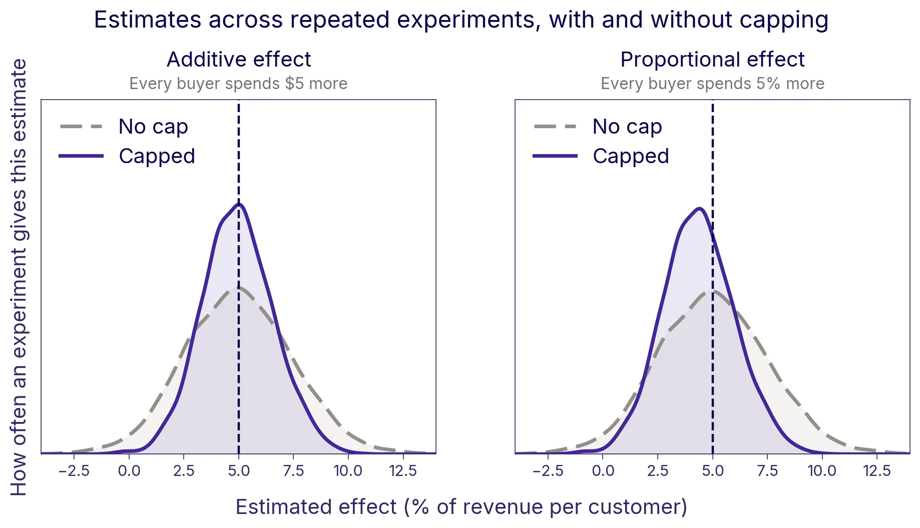
Why is this happening? Capping replaces the values of the buyers above the threshold with the threshold itself, in both arms. Whatever the treatment did to those buyers is erased. Their contribution to the estimate becomes the same number in treatment and in control, so it's zero.

So the cap removes whatever share of the effect the capped buyers carry. Under a proportional effect, buyers contribute in proportion to what they spend, so that's their share of revenue, 13% here. Under an additive effect they contribute equally, so it's their share of buyers, 1%. The same holds for other spending distributions, as the table further down shows.

That assumes your biggest spenders respond like everyone else (by the same amount or the same percentage). If the effect is more concentrated among them, capping erases most of it, and in the extreme the capped estimate shows nothing at all. They could also respond in the opposite direction, say a price cut that brings in small buyers while your biggest ones pay less for the same basket. In that case, capping removes a negative contribution and the capped estimate overstates the effect.

How much the bias under the proportional effect matters depends on what you use the estimate for. If you're deciding whether to ship, it rarely changes the decision, as the next section shows.

If you need the number itself, it's a bias-variance trade-off. The capped estimate is too low on average, but it varies less. When the effect isn't particularly concentrated in the tail, the capped estimate still comes closer to the true effect on average than the raw one does. The raw estimate comes closer only when the bias is large compared to the noise, for example with a feature that mostly affects your biggest buyers.

The bias also carries over to the confidence interval. It's a valid interval for the capped effect, not the uncapped one. As a result, it misses the uncapped effect more often than the stated 95%, and more so the larger the effect.

If you would like to check which customers your effect comes from rather than assume it, quantile treatment effects are the natural tool, alongside a segment analysis by pre-experiment spend. Compare the 90th percentile of spend between the two arms, then the 99th, and see where the difference appears. This works up to a point. To see the buyers the cap actually affects, you typically need to look further out than the 99th percentile, and that's where the quantile estimate becomes imprecise and the inference harder to get right. It's a useful exercise nonetheless.

A simpler check is to compare the raw and capped results, which GrowthBook shows in the Debug tab of the metric drilldown, and to add the same metric capped at a few different thresholds, which is easy with metric groups. That shows how much your estimate depends on the customers you cap, but not whether that part is a real effect or chance. We come back to what to make of it when the raw and capped results disagree.

Does capping increase power?

The point estimate might not, however, be the most important outcome of your experiment. If you're just making a shipping decision, what you care about is power. That is, the probability that a real effect is estimated as statistically significant. That depends on the standard error and the point estimate, together. For this purpose, the picture is actually looking quite good, even with the bias.

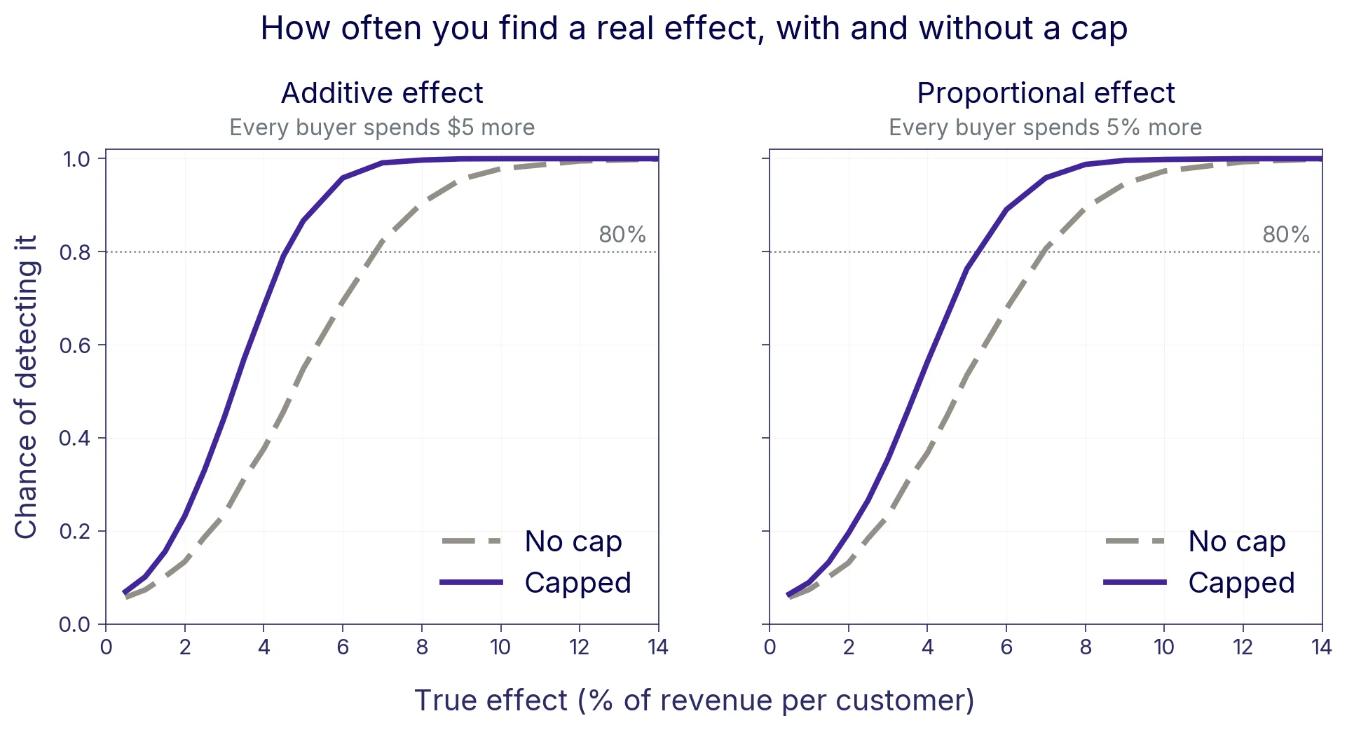
At a true effect of 5%, the raw estimate is significant a little more than half the time, i.e. roughly 50% power, whichever of the two effect types it is. Capped, the proportional effect, the one where the cap removes an eighth of the estimate, still has roughly 75% power. Losing an eighth of the effect and detecting it with 75% chance is probably better than keeping all of it and detecting it with only 50% chance. With the additive effect, the best case, capping increases power to almost 90%.

Hence, it comes down to what you want out of your estimate. If you need the number itself, for a forecast or a business case, the cap costs you some bias. Whether the lower variance makes up for that depends on your setting. If you need to decide whether to ship, you need power, and the cap gives you a lot of it for a modest price.

How deep should you cap?

All of that is for a cap on the top 1% of buyers. Whether that threshold is good for you depends on two distributions: the distribution of your treatment effect and the distribution of your outcome metric.

If the treatment effect is large for users at the top of the outcome distribution, capping deeper removes more of the effect. If the outcome distribution has a longer tail, the tail users contribute more noise to the estimate, and capping deeper improves precision more. Capping more deeply helps as long as it removes a larger share of the noise than of the effect.

So think carefully about what your treatment does to the tail users and check the distribution of your metric in the intended audience. If it's hard to make the case that your feature affects big spenders any more than regular users and you have a long tail, you can cap deeper.

In our example, moving the cap from the 99th to the 95th percentile of buyers takes the standard error from about two thirds of the raw one to about half. With an additive effect you keep almost all of the effect, and power rises from almost 90% to almost 100%. With a proportional effect the estimate falls from 87% of the true effect to 70%, and power barely moves, from roughly 75% to 80%.

That's not an argument for capping hard. Whatever the treatment did above the threshold is gone from the estimate, so the deeper the cap, the more of the effect it removes. At the extreme, a cap that reaches every buyer turns revenue per customer into a count of buyers, and an effect on how much people spend disappears from the estimate entirely. If zeros are counted when setting the threshold, that already happens at the 90th percentile of all customers when one in ten of them buys. Cap responsibly.

Does this hold for your data?

Your data might not look exactly like this, so I ran the same comparison across spending distributions where the top 1% of buyers hold anywhere from 3% to 30% of revenue. With a small tail, capping at the 99th percentile of buyers makes no difference. As the tail gets heavier, the power gain grows quickly, and the bias under a proportional effect grows more slowly.

So capping doesn't help when there's little tail variance to remove, as in the top row, where power barely changes. It hurts when the effect is concentrated among the buyers it caps. Otherwise, it increases power.

Your own numbers will differ, and that's what the capping explorer is for. Set it up to match your data, and see what a cap does to the estimate and to how often you find the effect. Then try a deeper cap, or a feature that affects your biggest buyers differently, and watch how the picture changes.

When raw and capped results disagree

Most platforms show you both the raw and the capped estimate, and sometimes one is significant and the other is not. When there's no real effect the two rarely disagree at all, less than 5% of the time in this example, and neither direction is more likely than the other. When there's a real effect the disagreement runs almost entirely one way: the capped estimate is significant and the raw one is not. That's what you'd expect, since the capped metric has the smaller standard error and becomes significant first.

So a capped-only result is usually a real effect that the raw metric is too noisy to confirm. The reverse case, raw significant and capped not, is rare. It means the difference between the arms comes from the customers above the threshold, and the two numbers alone can't tell you whether that's a real effect on your biggest customers or a few of them ending up in the same arm by chance. CUPED or post-stratification make the chance explanation less likely. Nonetheless, treat it as unconfirmed rather than as a win among your biggest customers.

Zeros and per-arm thresholds

"Cap at the 99th percentile" involves two further decisions, and they matter more than the percentile itself.

Whether zeros are counted. With one customer in ten buying, the 99th percentile of all customers affects the top 10% of buyers. That's probably more aggressive than you intended when selecting the 99th percentile, and it makes a difference. In this setting and with zeros excluded, the proportional-effect estimate drops to 87% of the true effect. With zeros counted, it drops to 59%. You might still gain power, but you're making a bolder assumption about the treatment effect on your best customers.

The fewer of your customers buy, the further down into your buyers the same percentile reaches. So ignore the zeros, and lower the percentile instead if you want to cap harder. Platforms differ on the default, so check what yours does.

Whether the threshold is computed on both treatment arms together or on each arm separately. Most of us have this one backwards. A single threshold for both arms seems fair, and giving each arm its own looks like judging them by different rules. But the single threshold is the more biased one: it gives the biggest buyers in both arms the same value, so the treatment effect on them cancels out. A per-arm threshold moves with the arm, so less of the effect is erased.

What per-arm capping costs is false positives. Two separately estimated thresholds differ by chance, and the usual standard error doesn't account for that, so the false positive rate goes from 5% to around 9%, and higher in heavier tails. Wicker (2026) shows this neatly.²

A standard error that accounts for the estimated thresholds fixes the false positive rate, but at least in this setting, you then get the same power as pooling or less. So per-arm only helps if you care about the point estimate itself, and then it's the same bias-variance trade-off as before: a little less bias for a little more noise.

To cap it off

Capping changes two things at once, and they depend on different things. The variance it removes depends on your spending distribution, the effect it removes depends on your treatment. The trade-off is good when the first is large and the second is small.

Most experiments are run to decide whether to ship something. If that's what you're doing, cap. Unless you expect your biggest buyers to be affected out of proportion to everyone else, the precision is worth more to you than unbiasedness.

Think carefully about how your treatment may affect customers differently. Quantile treatment effects can give you a hunch, but they get imprecise far out in the tail, which is where the cap acts.

If you need the point estimate itself rather than the decision, for a forecast or a business case, keep in mind that the capped estimate is biased by an amount your experiment can't show you. If you don't think the effect comes mostly from your biggest buyers, the capped estimate is still likely the one closer to the truth. CUPED and post-stratification reduce variance without adding bias, and they're worth using alongside capping too. Capping needs no pre-experiment data and targets the tail. CUPED and post-stratification work across the whole distribution, as far as your pre-experiment data allows.

Running efficient experiments isn't trivial, and all tricks come with caveats. I'm glad we cleared this one up a bit, so you can more comfortably reduce variance and speed up your experiments. Happy experimenting.

¹ This piece is about capping real values. If you're actually trying to remove erroneous data points, such as bots or test orders, then an absolute cap is probably the better tool. You use business context to set it at a value you can defend as implausible for a real customer.

² Till Wicker, "Winsorizing and Trimming in RCTs," Journal of Development Economics 182 (June 2026): 103815, https://doi.org/10.1016/j.jdeveco.2026.103815.

Appendix: how the simulation works

Each simulated customer has a latent score, drawn from a standard normal distribution. A customer buys during the experiment if the score is above 1.28, the 90th percentile of the standard normal, so that 10% of customers buy. Spend given buying is

rescaled so that the median buyer spends $60. Because spend is an increasing function of the score and only customers above the threshold buy, spend among buyers has a floor, at about $32, and a long right tail. Because it's a lognormal cut off from below, every moment of this distribution is finite. Over the range any single simulated experiment sees, though, its top end behaves like a power law with a tail index of about 2 (the Hill estimate over the top 1% of buyers), which is the point at which a true power law's variance becomes infinite.

Two treatment effects are simulated. Additive effect: every buyer's spend is increased by the same amount. Proportional effect: every buyer's spend is multiplied by a constant. For a 5% effect, the proportional effect multiplies spend by 1.05, and the additive effect adds 5% of average spend per buyer, about $5, so both raise revenue per customer by 5%. Two further effect types were simulated during the work and aren't shown: one on the extensive margin, where the buying threshold is lowered so that customers just below it start buying, and one concentrated entirely among the largest spenders.

Each replication draws a fresh population of 300,000 customers, so each experiment is a new sample from the same underlying distribution, not a re-randomization of one fixed population. It assigns every customer to treatment or control independently with probability one half, and applies the treatment to the treated customers. Revenue per customer is then estimated as the difference in means between the arms, with a Welch standard error, in two versions: on the raw values, and after replacing every value above the 99th percentile of the non-zero values in the pooled sample with that percentile. A result is called significant if the estimate is more than 1.96 standard errors from zero. Power is the share of replications in which that happens. The false positive rate is the same share when the true effect is zero. The Welch standard error of the capped estimate matches the actual spread of the estimates across replications, so the precision gain isn't a result of understating uncertainty. Power is estimated over 3,000 replications at each effect size, and every effect size is applied to the same 3,000 simulated populations and assignments.

The other results come from additional runs with the same generator and 300,000 customers per experiment, each with 1,000 to 2,000 replications: a sweep of the spending distribution, from one where the top 1% of buyers hold 3% of revenue to one where they hold about a third, covering both effect types and the zeros-included rule; the comparison of caps at the 99th and 95th percentiles of buyers; and the per-arm thresholds. For the per-arm cap, power is computed twice: once with the usual Welch standard error, and once with a corrected one equal to the actual spread of the per-arm estimate across replications with no effect.