Correlation vs. causation: What's the difference?

A chart can tell you that two numbers moved together. It cannot tell you what would have happened if you changed one of them.
That missing counterfactual is the difference between correlation and causation. Correlation summarizes an observed relationship. Causation answers an intervention question: if you deliberately changed X while holding the relevant alternative explanations in check, would Y change?
Product teams cross this boundary constantly. Activated users retain longer, customers who use integrations spend more, and accounts that adopt a new feature expand faster. Those patterns are useful. They are not yet proof that forcing the behavior will produce the outcome. High-intent customers may cause both adoption and retention, making the feature look more powerful than it is.
This guide explains how to read associations without dismissing them, how causal errors enter ordinary dashboards, and how randomized experiments turn a plausible story into evidence you can use for a decision.
Correlation describes association, not intervention
Correlation measures how variables vary together. A positive correlation means high values of one tend to accompany high values of the other. A negative correlation means high values of one accompany low values of the other. A value near zero indicates little linear association, although a strong nonlinear relationship may still exist.
A coefficient compresses a pattern
Pearson's correlation coefficient, usually written as r, ranges from -1 to 1. It captures the direction and strength of a linear relationship. It does not tell you the slope in business units, prove that the variables are independent when r is zero, or reveal whether extreme observations drive the pattern. The JMP statistics reference also stresses that pairwise correlation cannot account for an underlying third-variable relationship.
That is why a scatter plot should accompany the coefficient. The Khan Academy correlation lesson uses familiar examples to show that a relationship can be real in the data and still support a false causal story. Different datasets can share a correlation while having different shapes, clusters, and outliers.
For a product team, “feature usage and retention have r = 0.62” is an association statement. It says neither that increasing usage will improve retention nor how much retention would change. The coefficient may still be valuable for prediction, segmentation, instrumentation checks, or hypothesis generation.
Prediction can work without causation
A variable does not need to cause an outcome to predict it. Umbrella sales may predict rainy-day traffic even though umbrellas do not cause rain. A model can use device, session pattern, and account attributes to forecast churn without claiming that changing those attributes would prevent churn.
Problems arise when a team treats a predictive feature as an intervention target. A model might learn that customers who contact support frequently are more likely to renew because complex enterprise accounts both need support and have durable contracts. Reducing support contacts would not necessarily improve renewal. It might remove the help that keeps those customers successful.
Use predictive language for predictive evidence: “associated with,” “forecasts,” or “helps identify.” Reserve “drives,” “improves,” and “causes” for designs that justify an intervention claim.
Causation is defined against a counterfactual
Suppose an account receives a new onboarding flow and activates. The causal question is not whether activation occurred. It is whether that same account would have activated under the old flow at the same moment and under the same conditions. You can never observe both outcomes for one unit.
Causal designs construct a credible comparison group for that missing outcome. Randomized experiments do this by assigning similar units to control and treatment in expectation. Quasi-experimental methods do it through assumptions about cutoffs, timing, instruments, parallel trends, or matched comparison groups. In every case, the design carries the causal argument.
Build a testable causal claim
Learn how to define the population, treatment, exposure, metrics, and decision rule before an A/B test starts.
Watch the Webinar
Four mechanisms make correlation look causal
“Correlation is not causation” becomes useful only when you can name a plausible alternative explanation. Most misleading product correlations come from 4 mechanisms.
A confounder influences both variables
A confounding variable is a common cause of the apparent treatment and the outcome. Account maturity can increase both integration adoption and retention. Warm weather can increase both ice cream sales and swimming incidents. The observed variables move together because both sit downstream of something else.
The confounder may be measured, such as plan type, geography, or acquisition channel. It may also be unmeasured, such as motivation or organizational capability. Regression adjustment can address variables you measured correctly. It cannot automatically remove confounders that are missing, badly measured, or chosen after the outcome.
GrowthBook's existing guide to false causality and confounding explores how these hidden variables and Simpson's paradox can reverse an aggregate story.
Cause and effect run in the other direction
Heavy users often adopt more features. A dashboard may suggest that feature breadth creates engagement, while existing engagement actually creates feature discovery. Both directions may operate at once.
Time order helps: a cause must precede its effect. But sequence alone is not enough. A product launch preceding a revenue increase does not rule out seasonality, a promotion, or a competitor outage. Lagged correlations can narrow a theory without proving it.
Selection changes who appears in the data
Conditioning on a treatment-dependent event can manufacture an association. Imagine comparing revenue only among users who completed checkout. If a new flow changes who completes checkout, the selected treatment and control groups are no longer comparable. Revenue per purchaser might rise even while revenue per assigned user falls.
The same error occurs when analysts include only “active” users after a feature changes activity. Analyze the randomized population for the primary intent-to-treat estimate, or define activation before launch and use a method appropriate to the estimand.
Shared trends and chance create convincing patterns
Two metrics can rise because the product, traffic, and market are growing. Raw counts often correlate simply because both contain a time trend. Detrending, using rates with defensible denominators, checking seasonality, and comparing concurrent controls help expose this issue.
Chance becomes more dangerous as the number of metrics, segments, and time windows grows. If analysts search enough combinations, some will look impressive. Predeclared outcomes and multiple-comparison controls limit the freedom to draw a target around noise.
Randomization turns association into causal evidence
A randomized controlled experiment deliberately changes treatment and uses chance to assign eligible units. This breaks the systematic relationship between treatment and pre-existing characteristics in expectation.
Assignment must happen before treatment
Choose the unit that can independently receive the change: user, account, device, request, region, store, or another cluster. NIST describes a completely randomized design as one where treatment levels are randomly assigned to experimental units.
The unit must match the treatment. Randomizing teammates individually for a shared workspace feature creates interference because one person's experience can affect another's outcome. Randomizing accounts protects the boundary, but the analysis must then account for account-level assignment rather than treating every event as independent.
GrowthBook's guide to experimental units explains this connection between the assignment unit, independence, and valid uncertainty.
Exposure must represent the point of divergence
Assignment says what a unit would receive. Exposure records when the treatment could first affect behavior. Logging exposure at application startup may include users who never encounter the feature, diluting the estimate. Logging it after a treatment-dependent click selects on an outcome.
Place the event at the earliest point where variants diverge. Record the experiment key, variant, unit identifier, timestamp, and relevant implementation version. Then verify that exposure precedes measured outcomes and joins to the intended unit.
Outcomes and decision rules must be predeclared
Define one primary outcome, its numerator and denominator, attribution window, exclusions, minimum detectable effect, and stopping rule before opening results. Add secondary metrics for interpretation and guardrails for harms the primary metric might miss.
The CDC causal-inference teaching material describes randomized assignment as particularly strong evidence for causation. Digital experiments benefit from the same logic, but only if implementation and analysis preserve the assignment.
Randomization does not rescue a broken metric, missing exposure data, cross-variant contamination, or selective reporting. It provides a strong foundation whose assumptions still need verification.
Observational evidence can be useful without overclaiming
Some questions cannot be randomized. A team may need to evaluate a historical launch, a pricing change applied to all customers, a policy event, or a rare safety outcome. The correct response is not to discard the data. It is to match the claim strength to the design.
Use associations to generate and prioritize hypotheses
Correlations reveal where to investigate. If integration adoption is strongly associated with retention, ask what mechanism could connect them, which customer characteristics affect both, and whether adoption occurs before retention differences emerge. Interview customers, inspect sequences, and propose an intervention that changes adoption without changing everything else.
Then test the intervention. The experiment may show that guided integration setup changes retention, that it only helps a particular segment, or that adoption was merely a marker of committed customers. Any of those answers is more actionable than the original coefficient.
Stronger nonrandomized designs make assumptions visible
When an experiment is impossible, causal inference may use:
- Difference-in-differences: Compare outcome changes over time between affected and unaffected groups under a parallel-trends assumption.
- Regression discontinuity: Compare units just above and below a treatment cutoff when manipulation around the cutoff is limited.
- Instrumental variables: Use a source of treatment variation that affects the outcome only through treatment.
- Matching or weighting: Balance observed pre-treatment characteristics while acknowledging unmeasured confounding may remain.
- Interrupted time series: Look for a level or trend change at an intervention point while modeling seasonality and other events.
Each method replaces randomization with assumptions that need defense. A model's sophistication does not erase the design problem. The useful Hacker News discussion on causation beyond simple correlation reaches the same practical point: natural experiments and instruments can help when the variation approximates an independent intervention.
Triangulate when no single design can settle the question
Combine evidence with different failure modes. A product team might use observational sequences, customer interviews, a natural experiment from staggered rollout timing, and a smaller randomized nudge. Agreement across methods strengthens confidence because the same hidden bias is less likely to explain every result.
Do not collapse that into “proved.” Report the estimate, population, assumptions, uncertainty, and alternative explanations. Good causal communication tells the reader what design makes the claim credible and where it could still fail.
Audit causal language before it reaches a roadmap
The most practical safeguard is a short review that separates observation from intervention.
Ask what evidence the sentence actually contains
For any claim that X drives Y, ask:
- Were units randomly assigned to X, or was X observed?
- Did X occur before Y?
- Could a third variable affect both?
- Did selection into the analyzed sample depend on treatment or outcome?
- Were the outcome and analysis chosen before results?
- Does the estimate apply to the population and decision at hand?
If the design is observational, rewrite the sentence as an association unless a credible causal method and its assumptions are stated. “Accounts using 3 integrations retained at a higher rate” is accurate. “Adding 3 integrations improves retention” requires intervention evidence.
Check experiment health before reading the effect
For randomized tests, review allocation, pre-experiment balance, exposure coverage, identity joins, metric freshness, and concurrent changes. Sample ratio mismatch can signal assignment or tracking failures. Novelty, interference, and attrition can still make a short-term average misleading.
GrowthBook's experiment analysis workflow combines result interpretation with health checks, while warehouse-native experimentation lets data teams inspect the query logic behind metrics. Transparent SQL does not guarantee causality, but it makes the evidence chain auditable.
Make the decision proportional to uncertainty
A low-cost, reversible change can proceed on weaker evidence with monitoring. A pricing shift, safety-critical algorithm, or irreversible migration requires stronger identification, longer-term guardrails, and often replication. Practical significance matters alongside statistical evidence: a precisely estimated effect smaller than the cost of implementation is not a win.
The goal is not to eliminate uncertainty. It is to prevent an association from silently becoming a causal promise as it moves from dashboard to meeting to roadmap.
Treat correlation as a clue and causation as a design claim
Correlation is not the enemy of causal reasoning. It is often where causal reasoning starts. It identifies patterns, improves forecasts, and helps teams choose where an experiment could create the most learning.
The discipline is to keep 3 statements separate: what the data shows, what mechanism might explain it, and what design could test that mechanism. When those blur together, a compelling chart becomes an expensive product decision. When they remain distinct, observational data and randomized experiments reinforce each other.
Pick one important correlation in your product data. Draw at least 2 alternative causal diagrams, name the confounders and selection points, and design the smallest reversible intervention that distinguishes the stories. That is the move from “these metrics travel together” to “this change produced this outcome.”
Test the cause, not the story
Use GrowthBook to randomize product changes, measure trusted warehouse outcomes, and review the evidence behind the result.
Get StartedRelated Articles
CLI vs MCP: TLDR, it doesn’t matter as much as you think
Your agent should know how to do the job whichever interface it uses.
Your coding agent can already run terminal commands. Your product manager's assistant can connect to remote tools. Both need to inspect the same experiment, understand the same metric, and prepare changes to the same feature flag.
That creates a familiar question: should you give them a CLI or an MCP server?
The usual answers mix several concerns. A CLI is easy to compose with scripts. MCP gives compatible clients a standard way to discover and invoke tools. Skills can supply the instructions that make either route useful. None of those statements tells you whether the agent knows your release process or can distinguish a draft from a live change.
For GrowthBook, the choice has become smaller. We've built the agent layer around a REST API and reusable workflow skills, then made those available through different interfaces. Your choice of CLI or MCP no longer needs to determine which product workflow your agent can understand.
It still determines how the agent connects, executes requests, and handles credentials. This article explains that distinction, shows the same disabled-flag operation through both routes, and gives you a way to evaluate the integration you actually intend to use.
The debate combines three different questions
Start with a specific job: prepare a release control for a new checkout flow. The agent needs to know which project owns checkout, which environments exist, what the default behavior should be, and whether the proposed flag key already exists.
Choosing an interface answers only part of that job.
How can the agent reach the product?
A command-line interface lets an agent invoke a program in an environment where it has shell access. That program can make authenticated API requests and return data. You can also run the same commands yourself, put them in scripts, and preserve output for inspection.
The Model Context Protocol architecture connects a host application to servers through clients. An MCP server exposes capabilities that a compatible host can discover and call. The host might be a coding environment, a desktop assistant, or another agent application.
These categories overlap. A terminal-based agent can also be an MCP client. A local MCP server can be a process launched by that client. A remote MCP connection can work without the host giving the model a general-purpose shell.
So “terminal agent” doesn't automatically mean “use the CLI,” and “MCP” doesn't automatically mean “remote service.” Ask what access the runtime provides before choosing the adapter.
What procedure should the agent follow?
An API can expose a create operation without teaching an agent when to use it. A syntactically valid feature flag might still have the wrong project, an ambiguous key, or a default value that doesn't match the application.
That's the job of a skill: reusable instructions for a recognizable task. The Agent Skills format gives those instructions a portable structure, including a skill entry point and supporting references. A workflow can describe the context to inspect, the sequence to follow, and the evidence to return.
For the checkout example, useful guidance says to resolve environments, check the permanent key, choose a value type, and create the flag disabled. Merely exposing a create command leaves those decisions to the agent's general knowledge.
Skills are also useful when the right answer is to take no action yet. “Create a flag” and “design an experiment” are related requests, but they can require different objects and sequencing. An agent needs enough product guidance to make that distinction.
What context makes the procedure relevant?
Even a good playbook needs the current product state. The agent should inspect the objects in your GrowthBook organization and, when it is changing application code, the repository's SDK initialization and tests.
Those are different sources of context. GrowthBook supplies flags, experiments, metric definitions, and other authorized product resources. Your coding runtime supplies the application files it can access. An MCP connection doesn't by itself grant repository access, and a CLI doesn't by itself explain your metric definitions.
Evaluate the combination: access to the product, a maintained procedure, and enough context to apply that procedure. A comparison that changes all three at once cannot isolate the effect of CLI versus MCP.
GrowthBook puts the durable parts below the interface
We separated the agent layer into responsibilities that can be reused. The product API exposes operations. Skills explain workflows. The interface connects the agent to those two layers.
This is the architectural shift behind GrowthBook's agent experience. Instead of making every client integration carry its own interpretation of experimentation, we can share the interpretation and change how it is delivered.
The API provides the operations
GrowthBook's REST API makes product objects addressable. An agent can inspect a project, retrieve a flag, or perform an authorized operation against those objects.
The rebuilt API described in GrowthBook 4.4 uses shared schemas to support types, validation, and API documentation. The CLI is generated from the API definition. That reduces the amount of separately maintained command logic needed to expose product operations.
The OpenAPI specification explains the underlying principle: a machine-readable description can represent an HTTP API's paths, operations, inputs, and responses. Generation is useful because it derives another interface from that contract.
Generation doesn't mean any installed binary knows every future endpoint. The generated client still has a version, and your GrowthBook server still has a version. A self-hosted instance can lag behind the public documentation. Treat API compatibility as a deployment fact you verify.
Skills provide the workflow guidance
GrowthBook's feature-flags skill routes requests to more specific workflows. Creating a flag, inspecting dependencies, changing targeting, requesting review, and publishing a revision are separate procedures.
That structure lets the agent load the guidance relevant to the current job. The skill authoring guidance on progressive disclosure supports this approach: keep the entry point focused and place detail in references that are loaded as needed.
The benefit is maintainability as well as context management. A correction to a flag workflow can be made in the maintained skill rather than repeated across a series of tool descriptions and client-specific prompts.
There are two shell concepts to keep distinct. The generated growthbook CLI is a terminal interface to the product API. The skills repository also includes a small gb-call helper for making REST requests. Installing a skill doesn't make that helper a globally available command; its location depends on the installation. Both can reach the API, but their configuration and invocation are different.
MCP provides a thin bridge
The current GrowthBook MCP implementation exposes four tools: growthbook_list_skills, growthbook_read_skill, growthbook_api_read, and growthbook_api_write.
An agent discovers a domain, reads the relevant workflow, then makes API calls. It doesn't need a dedicated MCP tool for every product endpoint. Calls described as gb-call GET in a skill map to the read tool; mutating methods map to the write tool with the same path and body.
The bridge does not run the shell helper. It forwards authenticated requests. Product-side permissions and validation remain important because a small tool surface can still reach many operations.
Shared guidance also has a delivery boundary: the MCP server bundles skills when it is built, using a pinned source revision. A newly edited skill in the repository needs to be included in a subsequent server build before that server supplies it. “Shared source” is a maintainability claim, not a promise of instant synchronization.
Explore the shared flag workflows
Open the feature-flags skill to see the procedures that guide creation, targeting, reviews, and publishing. Bring the same workflow knowledge to the agent interface your team uses.
View the Flag Skill
The same disabled flag can use either route
The practical question is whether the interface changes the job. Let's create a Boolean flag called checkout-redesign, with a false default and every environment disabled.
This is an API example for a sandbox project, not an application integration tutorial. It creates a control object; your application still needs a correctly configured GrowthBook SDK to evaluate it. The feature flag documentation covers the product concepts behind that integration.
Connect and verify before preparing the write
For the terminal route, install the current GrowthBook CLI, configure a Personal Access Token through its interactive setup, and inspect the available command syntax:
Check that the active server and identity are the ones you intend to use. Prefer a tested, pinned CLI version in repeatable automation. Don't include a live token in a command you plan to share.
For an MCP route, the GrowthBook Cloud setup uses the hosted endpoint and browser OAuth. In a client using the documented mcpServers configuration shape, such as Cursor, add:
Complete the browser authorization and confirm tool discovery. Other clients can use a different configuration shape. Self-hosted GrowthBook users should follow the local stdio or self-hosted HTTP instructions rather than point a private instance at the Cloud service.
Next, let the connected agent discover the flag-creation workflow. These are tool-call parameters, shown separately in the order to invoke them:
The returned guidance should describe the prerequisites for creating the flag. If the workflow isn't present, resolve the server's bundled skill version before substituting instructions from an older integration.
Resolve real IDs and construct one payload
The flag-creation workflow checks existing keys, lists projects, and resolves environments. In the MCP client, invoke the read tool with each of these argument objects:
For the CLI route, perform that discovery with the corresponding command groups documented in the CLI command catalog:
Inspect each command's help if your installed version differs. The returned keys, project IDs, and environment IDs are the inputs to the payload below. In MCP, the equivalent read-tool arguments are:
Verify that checkout-redesign isn't taken, identify the sandbox project's ID, and enumerate every actual environment. These read responses determine the payload; don't treat example environment names as a complete inventory of your organization.
Save the following as flag.json, replacing <PROJECT_ID> and the environment keys with the discovered values. This example assumes the only environments are staging and production:
The API represents defaultValue as a string, even for a Boolean flag. Explicitly disabling each environment avoids relying on the organization's default state for newly created flags. Use a PAT for this example so the caller has a user identity for attribution.
Review the permanent key, project, value, and disabled states before submitting. If the intended job is an experiment, route to experiment design first instead of creating an unrelated flag and hoping to connect it later.
Submit once, then read the object back
With the CLI, the create command accepts a JSON body. In a Bash-compatible shell, inspect the request with dry run before submitting:
The first command previews a request; it doesn't prove the server will accept it. Run the second only after checking the preview and approving this creation. In PowerShell, use that shell's file-reading syntax rather than paste the Bash substitution unchanged.
The PowerShell equivalent, using the same reviewed file, is:
The same distinction applies: preview first, approve the specific creation, then submit. Neither command changes the application's deployed code.
Through MCP, call growthbook_api_write with the same payload serialized into its body string. Substitute the same resolved project and environment names:
Choose one creation route. Don't run both against the same key; they target the same product object, and the second creation should encounter an existing key.
Verify through the CLI get command:
Or invoke growthbook_api_read with:
Check the returned key, project, value type, default value, disabled state of every environment, and absence of unintended rules. Report those facts rather than “success.” No targeting or exposure change is included in this example.
Choose the route that fits the runtime
Once the procedure and API operation are shared, the remaining choice is operational. Where does the agent run? What can it execute? How does it authenticate? What does your team need to inspect afterward?
Shell access favors terminal composition
A shell-capable agent can run the CLI alongside repository tools, save structured output, and combine product inspection with local checks. That is useful when the job includes code changes, generated files, or a reproducible script.
For example, a flag audit can produce an inventory file while an engineer separately checks code references. The agent should preserve the association between the GrowthBook key and each repository reference. The final artifact can include both the product state and the proposed code diff.
The shell makes composition available; it doesn't make a workflow safe by default. A script can select the wrong profile or swallow an error. Decide which failures stop the workflow, where outputs are stored, and which steps need a reviewable artifact.
Remote tool access favors MCP clients
MCP is useful when the host already provides a tool connection but doesn't expose a terminal. A PM can inspect an experiment through a compatible assistant without installing a product CLI inside that assistant's runtime.
The MCP authorization specification defines an authorization framework for HTTP transports. GrowthBook Cloud uses browser OAuth, while local stdio configurations use credentials supplied to the process. Those are distinct deployment paths.
MCP also gives hosts a structured description of tools. The tool specification includes annotations such as read-only and destructive hints. Hosts can use those signals in their interaction design, but the signals are not an access-control boundary. The product must still enforce the caller's actual permissions.
Use a small decision table
| Your immediate requirement | Route to consider | What to verify |
|---|---|---|
| Combine product operations with local files and scripts | CLI plus maintained skills | Shell access, profile, installed version, structured output |
| Connect a compatible assistant without a shell | Hosted MCP | HTTP/OAuth support, identity, tools, bundled workflow |
| Keep requests inside a self-hosted deployment | CLI or self-hosted MCP | Network reachability, server version, credentials, trusted app origin |
| Reuse a procedure across different team clients | Shared skills through either route | Workflow revision, API compatibility, expected review artifact |
You can support more than one row. An engineer's CLI and a PM's MCP connection can operate on the same objects with different identities and permissions. Standardizing the workflow is often more useful than standardizing everyone's client.
Compare actual outcomes, not tool counts
Four MCP tools can address a large API. A large CLI command catalog can expose the same operations. Counting entries tells you little about whether an agent completed the intended job correctly.
Likewise, there is no universal token or speed result implied by the architecture. The client, model, instructions, response size, pagination, and number of requests all affect a real run. Measure the work you need instead of importing a result from an unrelated integration.
Keep the evaluation task constant
Use one sandbox project and one bounded task. For a read test, ask each route to find a named flag and identify its enabled environments, current revision, and relevant dependencies. For a write test, use separate temporary keys with the same reviewed disabled-flag requirements.
Give both runs the same expected output. Record whether each identified the correct objects, loaded the relevant workflow, handled missing data, and preserved the boundary between creation and exposure. Measure elapsed time and context consumption only alongside those correctness checks.
If one run gets rich workflow guidance and the other gets only a command name, you're testing the guidance as well as the interface. That can still be a useful product evaluation, but describe what changed.
Test failure behavior deliberately
Try a nonexistent object, an existing key, and a credential without the required permission. The agent should identify the failure and stop the dependent action. It should not invent an ID, silently pick another environment, or reinterpret a permission error as permission to retry with a broader credential.
The revision workflow adds another important test: multiple open drafts. When a chain of changes belongs in one revision, the agent must preserve its version rather than repeatedly ask for whichever draft is latest.
A creation receipt and a publication receipt are different artifacts. If your evaluation only checks that a request returned without error, it can miss the point where a proposed change became live or where a draft failed to include the intended edits.
Record the versions behind the result
Capture the CLI version, server version when available, client configuration, and the skill text or revision used. With MCP, inspect the guidance actually returned by the connected server. With installed skills, inspect the local instructions actually loaded.
That record makes a later regression diagnosable. A changed result may come from new guidance, a client update, a changed API, or different product state. “MCP became worse” is too broad to help you fix it.
Build workflows that survive the next client
The most useful consequence of GrowthBook's design is organizational. Engineers, PMs, and analysts can choose the agent surface that fits their work while referring to the same flags, experiments, and metrics.
An engineer can prepare a disabled flag from a terminal. A reviewer can inspect its draft in the app. An assistant connected through MCP can retrieve the same object and explain its state. The handoff should carry an ID, a revision where applicable, the proposed behavior, and the decision still required.
This is where the CLI-versus-MCP question loses much of its importance. Your release procedure doesn't need to be rewritten around each client. The product holds state; the API exposes operations; skills explain the work; the chosen interface delivers access.
Start with one inspection or sandbox creation. Require the agent to return a concrete object and its verified state. Then add the next workflow only when the current one is reliable enough for your team to review.
GrowthBook's feature flag platform gives that work a common place to live. The durable choice is how you connect release control and measurement to your team's process. CLI and MCP are ways to carry that process into the tools people already use.
Start with a common foundation
Set up GrowthBook for the flags, experiments, and metrics your agents will share. Then choose the CLI or MCP connection that fits each team member's work.
Get Started With GrowthBook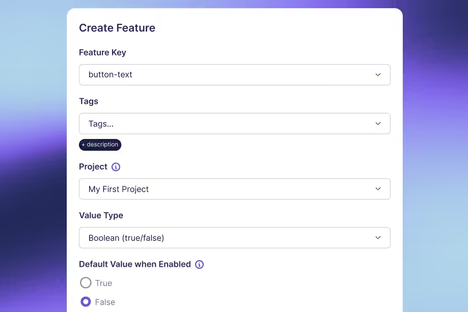
Standard deviation vs variance: Key differences for A/B testers
A metric can have wide user-to-user variation and still yield a precise experiment estimate.
That is why confusing standard deviation with standard error creates bad A/B testing decisions. A dashboard may show that users differ substantially while the average effect is estimated closely enough to guide a release. Those statements can both be true.
Variance and standard deviation describe spread. Variance works on a squared scale; standard deviation takes its square root to return to the metric's original units. Neither is automatically the uncertainty around an experiment result.
For A/B testers, the useful distinction is practical: use standard deviation to communicate outcome variability, use variance in the calculations that combine uncertainty, and inspect the standard error or interval for the treatment effect. Start by making sure all three describe the correct unit of analysis.
Understand the difference in units
Variance uses squared distances
Outcomes above and below a mean have deviations with opposite signs. Simply averaging those signed deviations gives zero. Variance avoids that cancellation by squaring each deviation before combining them.
The sample variance formula is s² = Σ(xᵢ − x̄)² / (n − 1), where x̄ is the sample mean and n is the number of observations. The symbol Σ means to add the terms across observations.
If the outcome is measured in seconds, variance is measured in seconds squared. That is mathematically useful but less intuitive for explaining a product experience. “Variance is 4 seconds squared” does not mean users differ by 4 seconds.
Standard deviation returns to the original scale
Standard deviation is s = √s². A variance of 4 seconds squared corresponds to a standard deviation of 2 seconds. Both describe the same dispersion, expressed on different scales.
Do not define standard deviation as the average absolute distance from the mean. That is a different measure. Squaring deviations gives large deviations more influence, and taking the square root afterward does not undo that weighting.
| Quantity | What it describes | Units for task time |
|---|---|---|
| Variance | Squared dispersion in outcomes | Seconds squared |
| Standard deviation | Outcome dispersion on the original scale | Seconds |
| Standard error of the mean | Sampling variability of an estimated mean | Seconds |
Neither variance nor standard deviation requires a normally distributed population merely to be calculated. Normality matters for particular interpretations and inferential procedures, not for the existence of these summaries when the required moments are finite.
Calculate both from the same observations
Work through a small dataset
Use four synthetic task times: 2, 4, 4, and 6 seconds. This tiny dataset is for arithmetic, not evidence about a real product or a basis for confident inference.
The mean is (2 + 4 + 4 + 6) / 4 = 4 seconds. Deviations from the mean are −2, 0, 0, and 2 seconds. Their squares are 4, 0, 0, and 4 seconds squared, totaling 8.
Treating these observations as a sample, the usual sample variance is 8 / (4 − 1) = 8/3, or about 2.667 seconds squared. The sample standard deviation is √(8/3), or about 1.633 seconds.
This is a useful check on a report. If someone describes the same sample's variance as 1.633, they have probably substituted the standard deviation. If the units are missing, the mistake is much harder to spot.
Choose sample or population formulas deliberately
If those four observations constitute the entire finite population you want to describe, population variance divides by 4: 8/4 = 2 seconds squared. Population standard deviation is √2, or about 1.414 seconds.
The population and sample distinction depends on what you are estimating. Having every recorded event from an experiment does not necessarily make those events the full population of future users or future conditions you care about.
The n − 1 denominator makes the usual sample variance an unbiased estimator of population variance under independent, identically distributed sampling with finite variance. It does not make the square root exactly unbiased for population standard deviation. Nor does it correct biased sampling or dependence between observations.
Verify the calculation with explicit function names
Python's statistics functions distinguish sample calculations from population calculations. With Python 3 installed, this standalone example requires no external packages or data:
The first line of output is 2.667 1.633; the second is 2 1.414. The different denominators explain the difference. Before comparing statistics from two tools, check their sample/population defaults and handling of missing values.
Find the noise you can reduce
Explore practical variance reduction methods, including metric design and CUPED, and the conditions that make each approach useful.
Read the Variance Reduction Guide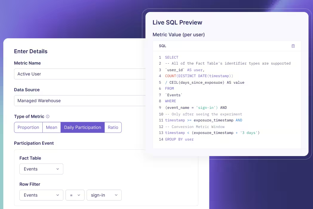
Use standard errors for experiment uncertainty
Distinguish users from estimated means
Standard deviation describes how users' outcomes vary. Standard error describes how an estimator would vary across repeated samples. For an independent sample, the estimated standard error of its mean is s / √n.
Suppose a user-level task-time metric has a sample standard deviation of 20 seconds among 10,000 independent users. The estimated standard error of the mean is 20/√10,000 = 0.2 seconds. Large differences between users coexist with a much smaller uncertainty around their average.
Collecting four times as many independent users would halve this standard error if the outcome variance stayed similar. It would not mechanically halve user-level standard deviation. The individual experience remains variable even as the estimated mean becomes more precise.
Combine arm variances before taking the square root
For independent treatment and control groups, a simple unadjusted difference in means has estimated variance s²ₜ/nₜ + s²꜀/n꜀. Its standard error is the square root of that sum. You do not add the two arm standard deviations and call the result the experiment's uncertainty.
Take a separate synthetic summary with 10,000 independent users in each arm and a 20-second standard deviation in both. The variance of the estimated difference is 400/10,000 + 400/10,000 = 0.08 seconds squared. Its standard error is √0.08, about 0.283 seconds.
If the observed treatment-minus-control difference is −1 second, an illustrative large-sample, unadjusted 95% normal interval is −1 ± 1.96 × 0.283, approximately −1.554 to −0.446 seconds. Negative values mean faster completion under this metric definition.
This example assumes independent groups and an appropriate large-sample approximation. It is not the exact output of GrowthBook's relative-lift, sequential, covariate-adjusted, or ratio-metric methods. GrowthBook's statistical details describe how the platform estimates effects and their uncertainty.
Avoid interpreting intervals as outcome ranges
That interval concerns the mean treatment effect. It does not say that 95% of individual users improved by between 0.446 and 1.554 seconds. An individual user's causal effect is a different quantity, and the experiment does not observe both potential outcomes for the same person.
Likewise, mean ± one standard deviation is not a universal statement about where 68% of users fall. That familiar interpretation depends on an approximately normal distribution. Skewed task times or revenue can look very different.
The frequentist confidence level describes the repeated-sampling coverage of the interval procedure under its assumptions. It is not a posterior probability assigned to a fixed realized interval.
Check what your metric actually measures
Match the variance to the randomization unit
If users are randomized and each contributes many requests, request rows are not automatically independent experimental units. Treating 100 requests from one person as 100 unrelated users can make uncertainty look smaller than it should.
Define the outcome at the intended unit or use a method that accounts for clustering. GrowthBook's aggregate data requirements are relevant when supplying precomputed summaries: the sample size, sum, and dispersion must correspond to the statistic and analysis method.
Two teams can report different standard deviations without either making an arithmetic mistake. One may summarize per-request latency while the other summarizes each user's average latency. They are describing different outcome distributions. Clarify the grain before comparing their numbers.
Paired measurements need another distinction. If the same users provide before-and-after outcomes, the measurements within each pair can be correlated. Analyze each user's difference or use an appropriate paired method; do not apply the independent-arm formula automatically. The paired-means framework treats those differences as the observations of interest. Pairing also does not remove time trends or establish causality by itself; the design still determines which comparison is defensible.
Inspect tails instead of deleting them casually
Large observations influence both variance and standard deviation. A few unusually long tasks can dominate a time metric; a few large purchasers can dominate revenue. Determine whether those values reflect valid behavior, instrumentation defects, retries, or unit errors.
A valid expensive user is not automatically an outlier to discard. Removing high values after seeing an experiment result can change the estimand and introduce selective analysis. Decide justified exclusions or transformations before interpreting the test.
Report complementary summaries when they answer useful questions: a histogram, median, or a relevant tail percentile can show what a single spread measure hides. Those summaries do not replace the mean effect if the mean remains the decision metric.
Keep units consistent across pipelines
Converting seconds to milliseconds multiplies every value by 1,000. Standard deviation also multiplies by 1,000, but variance multiplies by 1,000,000. A dramatic numerical variance increase can therefore be a unit conversion rather than a product regression.
For the four-value example, sample standard deviation becomes approximately 1,633 milliseconds and variance becomes approximately 2,666,667 milliseconds squared. The underlying task times have not changed. Store units with metric definitions and inspect them when comparing dashboards.
A lower variance caused solely by rescaling a metric does not create more statistical information. The effect size rescales too. Separate a numerical change in units from an actual improvement in the precision of your estimate.
Also avoid averaging standard deviations from daily reports and labeling the result a weekly standard deviation. The complete-period spread depends on both variation within days and differences between daily means. Keep the underlying observations or sufficient summaries that support the intended calculation. A simple average of displayed daily values generally loses information needed to reconstruct the full distribution.
Turn spread into a better testing plan
Define the outcome before planning the sample
Start with the metric definition: population, identity, aggregation, window, units, exclusions, and desired effect. Estimate variability from representative historical data at that same grain.
Historical variance is an input, not a guarantee. New traffic, a different user mix, or a changed measurement window can alter it. Explore plausible variance and effect-size assumptions rather than treating one historical number as exact.
Keep the two arm variances separate when appropriate. A treatment can change variability as well as its mean. The simple equal-standard-deviation illustration above is a teaching assumption, not a requirement that production groups have identical spread.
Reduce estimation noise without hiding behavior
CUPED and post-stratification use suitable pre-experiment information and covariates to improve effect estimation. CUPED stands for Controlled-experiment Using Pre-Experiment Data. Its value depends on useful predictive information and a valid implementation.
Adjustment can reduce uncertainty in the treatment effect without making real users' outcomes less variable. That distinction prevents a reporting error: a narrower adjusted interval is not evidence that customers now experience a more consistent product.
Also separate missing data from genuine zeros. A user with no purchase may correctly contribute zero revenue; a missing instrumentation event might represent an unknown outcome. Treating both identically can distort the mean and its variance before any statistical engine sees the data.
Report the right quantity for the decision
| Reader's question | Useful quantity |
|---|---|
| How much do individual outcomes differ? | Standard deviation, with distribution context |
| What enters this uncertainty calculation? | Variance at the correct analysis unit |
| How precisely is the effect estimated? | Standard error and an appropriate interval |
| Is the measured difference worth acting on? | Effect size, uncertainty, guardrails, and decision context |
For a clear experiment readout, show the metric's unit and analysis grain, the estimated effect, and its appropriate uncertainty interval. Add outcome spread when it helps readers understand the population or diagnose a noisy metric.
GrowthBook's experimentation platform brings defined metrics and statistical analysis together. A trustworthy interpretation still starts with your measurement choices: describe spread with standard deviation, calculate with variance where required, and judge precision using the estimator's uncertainty.
Build a clearer experiment readout
Connect your metrics to GrowthBook and evaluate effects with the analysis method and measurement definitions your team has chosen.
Get Started With Experimentation
Catching 80 defects means little until you know how many defects existed.
Suppose a detector flags 125 suspicious software changes. Engineers inspect them and confirm 80 real defects. That tells you something about alert quality, but it does not tell you how many defects the detector missed. To calculate true positive rate, you need the actual positives outside the alert queue too.
True positive rate, or TPR, measures the share of actual positive cases that a system correctly identifies. It is also called recall or sensitivity. The formula is TP / (TP + FN), where TP means true positives and FN means false negatives.
The arithmetic is simple. Choosing the right population, labels, threshold, and denominator is the difficult part. This guide works through an engineering example, distinguishes neighboring metrics, and explains what changes when the “test” is an A/B experiment rather than an item classifier.
Start with actual positives, not alerts
Define the positive class
“Positive” means the condition you want to detect. It does not necessarily mean a good outcome. In a defect detector, positive means a real defect. In a spam filter, it means spam. Write that definition before calculating anything.
A true positive is an item that is actually positive and predicted positive. A false negative is actually positive but predicted negative. Those two groups together form the denominator: all actual positives in the evaluation sample.
The recall definition is therefore conditional on actual class membership. TPR asks, “Among the real defects, what proportion did we catch?” It does not ask, “Among the alerts, what proportion were real?”
Fix the unit and observation window
Choose a consistent evaluation unit. A code change, an individual finding, and a repository are different units. If one change generates 12 duplicate alerts, counting alerts in the numerator and changes in the denominator produces a meaningless rate.
For the example, each unit is one code change, evaluated once by one fixed detector version at one fixed threshold. An independent review process eventually labels each change as defective or not defective. The observation window is long enough for those labels to mature.
This resembles the discipline needed when defining experiment metrics: the event, identity, time window, and denominator must describe the same question. A correct formula applied to incompatible counts still gives the wrong answer.
Calculate TPR from the confusion matrix
Put every evaluated item in one cell
Consider an original synthetic evaluation of 1,000 code changes. Reviewers establish that 100 contain a defect and 900 do not. The detector catches 80 defects, misses 20, and incorrectly flags 45 nondefective changes.
| Actual label | Predicted positive | Predicted negative | Total |
|---|---|---|---|
| Defective | 80 true positives | 20 false negatives | 100 |
| Not defective | 45 false positives | 855 true negatives | 900 |
| Total | 125 | 875 | 1,000 |
Read the labels rather than relying on cell position. Libraries and reports can arrange axes differently. The scikit-learn confusion matrix convention uses actual classes on rows and predicted classes on columns, with class order also affecting where each value appears.
Check the totals before calculating rates. The four cells sum to 1,000. True positives plus false negatives sum to 100 actual defects. Predicted positives total 125, which is a different denominator.
Divide detected positives by all actual positives
The calculation is:
TPR = TP / (TP + FN) = 80 / (80 + 20) = 80 / 100 = 0.80 = 80%.
Interpret it in words: the detector caught 80% of the actual defects in this evaluation sample. It missed 20%, so the false negative rate is 20%. For a binary task with complete labels, TPR and false negative rate sum to 100%.
Do not divide 80 by 1,000. That would measure true positives as a share of all evaluated changes, not recall. Do not divide 80 by 125 either. That is precision, which answers the alert-quality question.
The result describes this sample and threshold. It does not establish that every future workload will have the same recall, or that all defect categories are equally detectable. Keep the counts beside the percentage so readers can see the support behind it.
Handle zero positive support explicitly
If the sample contains no actual defects, TP + FN equals zero. Sample TPR is undefined. Returning 0% would imply the detector missed known defects; returning 100% would imply it successfully found them. Neither interpretation is supported.
Software libraries need a practical zero-division convention. That convention can return a placeholder or warning, but it does not create evidence. Report “TPR unavailable: zero actual positives” and preserve the support count. A pipeline can then distinguish an unevaluable slice from measured poor performance.
Check the experiment error risks
See how power, repeated checks, and multiple comparisons affect the reliability of experimental decisions beyond a single classifier score.
Read the False Positives GuideCompare TPR with precision and false positives
Keep the denominators visible
For the same 1,000 changes, the other common metrics tell different stories:
| Metric | Calculation | Result |
|---|---|---|
| True positive rate / recall | 80 / 100 actual positives | 80% |
| Precision | 80 / 125 predicted positives | 64% |
| False positive rate | 45 / 900 actual negatives | 5% |
| Specificity | 855 / 900 actual negatives | 95% |
| Accuracy | (80 + 855) / 1,000 changes | 93.5% |
The classification metric definitions differ because they condition on different populations. Here, 36% of alerts are false, but the false positive rate is 5%. Calling both numbers “the false positive rate” hides the operational distinction.
Accuracy can also look reassuring in an imbalanced population. A detector that labels all 1,000 changes nondefective would be 90% accurate while detecting none of the 100 defects. TPR exposes that failure, though it still needs the false-positive side of the picture.
Choose a threshold for the decision
Suppose a stricter threshold, evaluated on the same labeled changes, catches 60 defects and incorrectly flags 10 nondefective changes. Its TPR is 60%, its precision is about 85.7%, and its false positive rate is about 1.11%.
This threshold reduces the review queue from 125 changes to 70. It also misses 40 defects instead of 20. Whether that tradeoff is acceptable depends on the consequences of a missed defect, the review team's capacity, and what action follows an alert.
A ROC curve plots TPR against false positive rate across thresholds. It helps compare operating points. It does not pick the operational threshold for you, and an area-under-curve summary does not specify the queue size at the threshold you intend to deploy.
If you tune thresholds using the same labels you later report as a final evaluation, the score can be optimistic. Use separate validation and held-out evaluation data, or another defensible evaluation design, and freeze the decision rule before the final assessment.
Specify the action at each threshold too. A low-confidence finding might create a suggestion, while a high-confidence finding might block a merge. Those are different interventions with different error costs. One aggregate recall figure should not imply that every detected item received the same treatment.
Make sure the labels can support the claim
Audit predicted negatives too
If engineers review only alerts, you can estimate precision within the reviewed alert population. You cannot directly count missed defects among unreviewed negatives. Assuming those changes are clean makes FN artificially small and TPR artificially high.
An evaluation may need independent review of a representative sample of predicted negatives, delayed incident labels, or a curated benchmark with known defects. Each approach has limits. Incident labels miss undetected failures; curated examples can differ from ordinary production work.
If the evaluation oversamples suspicious changes or certain repositories, report that design. Use appropriate weighting when estimating performance for the real workload. A simple unweighted confusion matrix describes the sampled dataset, which may not represent the deployed population.
Preserve uncertainty and segment support
An 80% estimate based on 4 detected defects out of 5 is much less precise than one based on 800 out of 1,000. The important sample size for recall is the count of actual positives, not just the total number of changes evaluated.
Report positive support by important slices, such as language, defect category, or repository type. A high pooled TPR can hide weak performance on a rare but expensive failure mode. At the same time, avoid declaring tiny slices definitively better or worse from a few examples.
Counts alone do not make observations independent. Many similar changes from one repository can share a common pattern. Use uncertainty methods that fit the evaluation design rather than assuming every row is an unrelated trial.
Separate label delay from label absence
A recently deployed change might appear nondefective because nobody has had time to find the bug. Treating it as a confirmed negative gives the newest cohort a different labeling standard from older cohorts.
Define when an item becomes eligible for evaluation and track unresolved labels separately. Keep model version, threshold, label version, and observation dates with the result. That makes a later score change interpretable: you can tell whether the detector changed, the workload changed, or the labels matured.
For a warehouse-native measurement workflow, these definitions belong in the underlying data model. Joining model decisions to review outcomes still requires identity and time alignment; a queryable warehouse does not automatically resolve ambiguous ground truth.
Keep comparable populations together
When comparing detector versions, evaluate them on the same held-out cases where possible. Otherwise, an apparent recall improvement could come from an easier mix of defects. Preserve a breakdown of new, removed, and unchanged cases so reviewers can see what changed between evaluations.
When combining reports, add the underlying TP and FN counts for nonoverlapping, consistently defined populations, then calculate the pooled rate. An unweighted average of repository percentages answers a different question because it gives a tiny repository the same influence as a large one. Either summary can be useful, but label the weighting explicitly.
If the same change appears in several reports, deduplicate or model that repeated observation before pooling. Repeated scans do not create additional independent defects. Keep an audit trail from the final counts back to the evaluated item identifiers so a suspicious rate can be investigated.
Connect detection quality to product decisions
Distinguish classifier recall from statistical power
In hypothesis testing, statistical power is the probability that a testing procedure rejects the null when a specified alternative is true. It is a repeated-test detection probability, depending on assumptions such as effect size, variance, sample size, and decision rule.
That is related to the idea of detecting a real signal, but it is not the same dataset as a labeled-item confusion matrix. In an ordinary A/B program, you do not observe the true causal effect of every experiment with certainty. Dividing declared winners by all experiments does not reveal a ground-truth TPR.
Power planning asks how often your procedure would detect a particular real effect under its assumptions. A classifier evaluation asks how many labeled positives were detected in the evaluated sample. Keep those questions separate when discussing GrowthBook's statistical methods.
Evaluate the intervention as well as the detector
An improved offline detector can still create a worse product workflow. More alerts might overwhelm engineers, delay releases, or catch defects too late to matter. Conversely, a modest recall change might be valuable if it catches the failures with the highest operational cost.
When appropriate, use randomized experiments to evaluate the downstream intervention: which review experience helps teams resolve defects, with what delay and cost? Keep detector recall, review workload, and product outcomes as separate measures.
GrowthBook's experimentation platform can analyze defined outcomes from such tests. Your team supplies reliable assignment, exposure, labels, and metric definitions. Neither a high TPR nor a significant product result eliminates the need to inspect the other evidence.
Use a repeatable reporting checklist
Before sharing a TPR number, state the positive class, evaluation unit, detector version, threshold, and label process. Show TP and FN beside the rate. Include precision or false positive rate so readers can assess the workload created by detection.
Then ask whether predicted negatives were evaluated, whether labels had time to mature, and whether the sample reflects the population where you will act. Mark zero-support slices unavailable and explain material gaps in coverage.
The useful result is a statement someone can audit: “At this threshold, the detector found 80 of 100 labeled defects in these 1,000 evaluated changes, while producing 45 false alerts.” That is a clearer basis for a decision than “our model is 80% accurate.”
Measure what the change delivers
Connect your data and defined metrics to GrowthBook to evaluate how a product or workflow change affects the outcomes your team cares about.
Start Measuring With GrowthBookReady to ship faster?
No credit card required. Start with feature flags, experimentation, and product analytics—free.